Lineweaver-Burk Plot - Online Tutor, Practice Problems & Exam Prep

The Lineweaver Burk equation, derived from the Michaelis Menten equation, provides a linear representation of enzyme kinetics, allowing for easier interpretation of data. In a Lineweaver Burk plot, the y-axis represents the reciprocal of the initial reaction velocity (1/v₀), while the x-axis shows the reciprocal of substrate concentration (1/[S]). The slope of the line is the ratio of the Michaelis constant (K_m) to V_max, with the y-intercept indicating 1/V_max and the x-intercept as -1/K_m. Understanding these components is crucial for analyzing enzyme behavior.

Lineweaver-Burk Plot

In this video, we're going to begin our discussions on Lineweaver-Burk plots by first introducing the Lineweaver-Burk equation. So recall from our previous lesson videos that the Michaelis-Menten equation describes the rectangular hyperbola that we see in a Michaelis-Menten enzyme kinetics plot. And so the Lineweaver-Burk equation also describes enzyme kinetic data that we see forming a line in a Lineweaver-Burk plot. And so the good thing about the Lineweaver-Burk equation is that really it's nothing new. We can pretty much say that the Lineweaver-Burk equation is the reciprocal of the Michaelis-Menten equation. So really, we can take the Michaelis-Menten equation and simply invert the equation or take the reciprocal of it, and then do a little bit of algebraic rearrangement to obtain the Lineweaver-Burk equation, which is shown right over here. So notice that the Lineweaver-Burk equation has the same exact enzyme kinetics variables as the Michaelis-Menten equation that we already covered. So they both have the initial reaction velocity, the kilometers, the \( V_{\text{max}} \), and the substrate concentration.

And so if we take a look down below at our image, notice that on the left here we have the Michaelis-Menten equation that we're already familiar with from our previous lesson videos. And so if we want to obtain the Lineweaver-Burk equation without having to commit it to memory, all we need to do is take the reciprocal of the Michaelis-Menten equation, and the reciprocal just means to essentially invert the equation. Now, if we invert one side of the equation, we also have to invert the other side of the equation. And so let's go ahead and start with this left side over here. So if we take the reciprocal of the initial reaction velocity, that's going to be inverting it, so what we're going to be left with on the left side is \( \frac{1}{\text{initial reaction velocity}} \). So now that we've taken the reciprocal of the left side, we can take the reciprocal of the right side over here. And so taking the reciprocal of the right side is essentially just going to be taking the denominator or what's on the bottom and placing it on top. And it's going to be taking the numerator, or what's on top, and placing it on the bottom. And so that's exactly what we're going to do when we take the reciprocal here. So now, we're going to take the bottom which is Kilometers plus substrate concentration and put that on the top. So we're going to have Kilometers plus substrate concentration on the top, and then, of course, on the bottom down here, what we're going to have is what used to be on the top. So that's going to be the \( V_{\text{max}} \times \) substrate concentration. So that is essentially the reciprocal of the Michaelis-Menten equation. Now, all we need to do is 2 steps of algebraic rearrangement. So recall that when we have addition going on in the numerator, that we can actually separate out these two components. We can separate the kilometers from the substrate concentration, as long as they both have their own denominator. And so that's exactly what we see down below. Notice that the kilometers is now separated from the substrate concentration. The addition is still here, but they both have their own set of the same common denominator. And so, notice that with this expression over here, \( \text{max} \). So this expression right here simplifies to just \( \frac{1}{V_{\text{max}}} \). And then, notice that this expression over here, we can actually take the \( k_m \) and the \( V_{\text{max}} \) right here and separate it from \( \frac{1}{\text{substrate concentration}} \), and that's exactly what we see down below. We have the \( \frac{k_m}{V_{\text{max}}} \times \frac{1}{\text{substrate concentration}} \). And really, that is it. That allows us to get the Lineweaver-Burk equation, which I'll admit at first glance looks pretty complicated, but we were able to obtain it just by taking the reciprocal of the Michaelis-Menten equation that we're already familiar with and doing 2 steps of algebraic rearrangement.

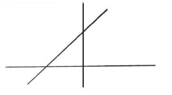
Now, again, this Lineweaver-Burk equation appears to be pretty complicated, but trust me, it's definitely not as complicated as it looks. And that's because it's no surprise that the line Weaver-Burk equation actually resembles the equation of a line. And, of course, we all know that the equation of a line is \( y = mx + b \). So, notice over here on the right side, we have the equation of a line, which is, again, \( y = mx + b \). And so, just like we can substitute in enzyme kinetics variables into a rectangular hyperbola equation to get the Michaelis-Menten equation from our previous lesson videos, we can also substitute in enzyme kinetics variables into the equation of a line to get the Lineweaver-Burk equation. And so notice that the \( y \) in our equation here is just going to be substituted with exactly what is on the \( y \)-axis of a Lineweaver-Burk plot, which is the reciprocal of the initial reaction velocity. Now, we know that the \( m \) is just going to be the slope of the line. And so, in the Lineweaver-Burk equation, the slope is equivalent to the ratio of the Kilometers over the \( V_{\text{max}} \). Now, the \( x \) is going to be exactly what we find on the \( x \)-axis of our Lineweaver-Burk plot, which is going to be the reciprocal of the substrate concentration. And then, of course, the \( b \) here is going to be the \( y \)-intercept of our line, and the \( b \) or the \( y \)-intercept in the Lineweaver-Burk plot is just gonna be \( \frac{1}{V_{\text{max}}} \). And so you can see here how the Lineweaver-Burk equation really does resemble the equation of a line, and that's why the Lineweaver-Burk equation describes the line that forms on a Lineweaver-Burk plot, and we'll talk about Lineweaver-Burk plots in our next lesson video, so I'll see you guys there.

Lineweaver-Burk Plot

So now that we've introduced the Lineweaver Burk equation in our last lesson video, in this video, we're going to introduce the Lineweaver Burk plot, which is really just another way to plot enzyme kinetics data. And so recall from our previous lesson videos, we had an enzyme kinetics plot in many of our videos and in the enzyme kinetics plot, we had the initial reaction velocity on the y-axis and the substrate concentration on the x-axis, and we know that Michaelis-Menten enzymes will form this rectangular hyperbola shape on this curve, which is definitely more complicated of a shape than a straight line. And so, instead of getting a rectangular hyperbola shape, the Lineweaver Burk plot, of course, is going to get a line, and so that's somewhat of an advantage of Lineweaver Burk plots that we're able to interpret the data just using a very simple straightforward line. And from this straight line that we get on a Lineweaver Burk plot, we're able to obtain the values for both the theoretical maximum velocity, \( v_{\text{max}} \), as well as the Michaelis constant \( K_m \). And again, these are both able to be determined from the straight line of a Lineweaver Burk plot. Now, it's also important to note that sometimes Lineweaver Burk plots are also referred to as double reciprocal plots and the reason that they are referred to as double reciprocal plots is because notice that on the plot, there's going to be a bunch of reciprocals. And so notice that instead of having the initial reaction velocity on the y-axis, on a Lineweaver Burk plot, notice that on the y-axis what we have is the reciprocal of the initial reaction velocity. And so that's what we're saying here is that we plot the reciprocals of both the initial reaction velocity as \( \frac{1}{v_0} \), here, but we also plot substrate concentration. So instead of plotting the substrate concentration, a Lineweaver Burk plot plots the reciprocal of the substrate concentration or one over the substrate concentration on the x-axis. And so, when, scientists do this, when they plot these double reciprocals, they're able to turn their data into a linear format. And so, what's important to note, as we kind of already mentioned in our last lesson video, is that the slope of the line that forms, so notice here, the line that we get here, the slope of this line in a Lineweaver Burk plot is going to be the ratio of the Michaelis constant, \( K_m \), over the \( v_{\text{max}} \). So essentially \( \frac{K_m}{v_{\text{max}}} \) will be equal to the slope of the line. And so notice over here on the left, what we have is the Lineweaver Burk equation that we introduced in our last lesson video and we know that it resembles the equation of a line. So we know that this reciprocal here is going to be the y of our line and we know that it's found on the y-axis for that reason. And so, we know that \( m \) here as we said up above, we know the \( m \) is going to be our slope and the slope of the line in a Lineweaver Burk plot is just going to be the ratio of the \( K_m \) over the \( v_{\text{max}} \). So this here, is going to be the \( m \), which means that the \( x \), so the \( m x \), is going to be the reciprocal of the substrate concentration and that's what goes on the x-axis of our plot. So, that's what goes down here, one over substrate concentration. And then it's gonna be plus \( b \). And we know that the \( b \) is going to be the y-intercept, which is pretty much where our line crosses the y-axis. So where our line crosses the y-axis is right at this point and that's why it's called the y-intercept or \( b \). And so the y-intercept is just going to be the reciprocal of the \( v_{\text{max}} \) or \( \frac{1}{v_{\text{max}}} \). And so, here what we can see is that the, y-intercept here is going to be, \( b \) and that's going to be \( \frac{1}{v_{\text{max}}} \), so we can write that in here, \( \frac{1}{v_{\text{max}}} \). The x-intercept, recall, is just where our line crosses our x-axis. So where those two points meet is going to be right here, and so this is going to be our x-intercept. And the x-intercept is also going to be the reciprocal, it's going to be the reciprocal of the \( K_m \), however. And it's gonna actually be the negative reciprocal, so it actually has a negative sign, negative one over \( K_m \), whereas none of our other reciprocals have a negative sign. And the reason that it has a negative sign is because notice that our x-intercept here is falling into the negative region of our plot. So here's 0, here are the positive numbers, and then to the left are the negative numbers and so because the x-intercept falls into the negative region that's why it has a negative here. And so of course we already said that the slope of this line here is going to be \( m \) and we said that it's going to be the ratio of the \( K_m \) over the \( v_{\text{max}} \), so we can indicate that here as well. \( \frac{K_m}{v_{\text{max}}} \). And so really these are the most important components that we need to take note of when it comes to a Lineweaver Burke plot. Now one additional thing that I want you guys to notice is that, notice that over here on this part of our line, that it is a solid line, but over here what we have is a dotted line. And so, the reason for that is because notice that, the, in order to get into this region over here where this dotted line is, we're actually gonna need to have negative negative, substrate concentrations to get over here. And, in reality, we're not able to get negative substrate concentrations. The lowest substrate concentration that we can get is 0 and so, this here, we're never gonna actually have data that falls into this region of our graph, so it's never gonna fall into that region. Our data, that we collect from an experiment is always gonna fall over here, which is why we have this solid line here. And again, that has to do with we we can only have positive substrate concentrations. And so, the data will fall over here, but we can always draw an imaginary line, so that's what this really is, an an imaginary line that extends and where this imaginary line crosses the x-axis, that's going to be the x-intercept here where we can derive the \( K_m \) from. And so you can see, as we mentioned up above, that from this straight line here, we're able to derive both the values for the \( v_{\text{max}} \) and the \( K_m \), and there's different ways that we can do that. We can do it through the slope because it has the \( K_m \) over the \( v_{\text{max}} \). We could do it through the y-intercept, which has, just the reciprocal of the \( V_{\text{max}} \), and we can do it through the x-intercept. And so, just by being familiar with the equation of a line, the Lineweaver Burk plot, the Lineweaver Burk equation, I'm sorry, and the Lineweaver Burk plot, we're able to solve a lot of problems that, teachers, like to ask on your biochemistry exam. So moving forward, we're gonna talk even more about, Lineweaver Burk plots to break them down even further. But this is a good initial introduction to Lineweaver Burk Plots, and in our next lesson video, we're going to, focus more specifically on these intercepts, the y-intercept, as well as the x-intercept. So I will see you guys in that video.

Lineweaver-Burk Plot

Alright. So now that we've introduced both the Lineweaver-Burk equation and the Lineweaver-Burk plot, in this lesson video, we're going to focus specifically on the y and the x intercepts of a line on a Lineweaver-Burk plot. The reason that we want to focus so much attention on the y and x intercepts is because the most important information on a Lineweaver-Burk plot is actually revealed through these intercepts of the line. That's because the y intercept and the x intercept are capable of revealing the Vmax and the K_m of an enzyme. But hang on, not so fast, because the intercepts do not directly reveal everything; everything is the reciprocal, including the intercepts. And so this means that the y intercept is going to reveal the reciprocal of the Vmax. Essentially, the y intercept is going to be 1V_max. If we want to get the V_max from the y intercept, then we need to take the reciprocal of the y intercept. Now, similarly, the x intercept is also the reciprocal. Instead, the reciprocal is going to be of the K_m and not of the V_max. We also need to recall from our previous lesson video that the x intercept on a Lineweaver-Burk plot will always fall into the negative region of the x-axis, which means that the x intercept is always going to have a negative value and that it's always going to be the negative reciprocal of the K_m, which is why we have -1K_m.

Also recall from your previous math courses, and chemistry courses, that the y intercept is going to be where the line intercepts, or crosses, the y-axis, and that can only happen when the value of x is equal to 0. And, of course, the x intercept is going to be exactly where the line intercepts or crosses the x-axis, and that can only happen when the value of y is equal to 0. If we take a look up at our Lineweaver-Burk plot from our previous lesson videos, recall that the y-axis is the vertical axis here, and the x-axis is the horizontal axis. The y intercept shown here is going to be exactly where our line crosses the y-axis, the vertical y-axis, which is right at this point right here. One way that helps me distinguish between the y and x intercepts and what they reveal, is that I know that on an enzyme kinetics plot, whether it be a Michaelis-Menten enzyme kinetics plot or a Lineweaver-Burk plot, this y-axis I know is always associated with reaction velocity, and so it's no surprise that the y intercept, which is associated with the y-axis, is also related to a reaction velocity, more specifically, the maximum reaction velocity. We know already that the y intercept is going to be a reciprocal on a Lineweaver-Burk plot since these plots are also known as double reciprocal plots and pretty much everything is the reciprocal, including these intercepts.

For similar reasoning, I know that the x intercept is always going to be associated with the x-axis, which is where our line crosses the x-axis, which is right at this position on this plot. And I know that the x intercept is always associated with a substrate concentration because it is a Michaelis-Menten plot or a Lineweaver-Burk plot, so the x intercept for that reason has to be associated with a substrate concentration, not a reaction velocity. Recall that the K_m is a substrate concentration, not a reaction velocity. And, of course, again, the x intercept we know is going to be a reciprocal because Lineweaver-Burk plots are double reciprocal plots. So it's the reciprocal of the K_m. And again, recall that the x intercept always will fall into the negative region when it's a Lineweaver-Burk plot. And that means that the x intercept is actually going to be the negative reciprocal of the K_m. Moving forward, we'll be able to get a lot more practice, focusing on these y and x intercepts and the information that they reveal. So that concludes this lesson and I'll see you guys in our next video.

To determine the V_max from a Lineweaver-Burk plot you would:

• A. Multiply the reciprocal of the x-axis intercept by -1.
• B. Multiply the reciprocal of the y-axis intercept by -1.
• C. Take the reciprocal of the x-axis intercept.
• D. Take the reciprocal of the y-axis intercept.

A Lineweaver-Burk plot generates a line with the following formula: y = 0.3x + 0.4. What is the K_m?

• A. 0.3
• B. 0.4
• C. 0.75
• D. 2.5

Consider the equation for the line on the following Lineweaver-Burk plot: y = 6x + 3

A) What is the K_m for the corresponding enzyme?

a) -2 mM 

b) 18 mM 

c) 2 mM 

d) 9 mM

B) What is the V_max for the corresponding enzyme?

a) 0.333 mM/s 

b) 9 mM/s 

c) -6 mM/s 

d) 18 mM/s

• A. -2 mM
• B. 18 mM
• C. 2 mM
• D. 9 mM

Suppose the data on the right is plotted onto a Lineweaver-Burk plot to obtain a straight line.

A) What is the value of the y-intercept of the line? ____________

B) What is the value of the x-intercept of the line? ____________

Alright. So this practice problem wants us to consider the following enzyme-catalyzed reaction shown right here, where we have substrate A being converted into product B. It says, suppose that the enzyme kinetic data for this reaction, which is shown in this chart right here down below, is actually inverted and plotted onto a Lineweaver-Burk plot to obtain a straight line. And so, notice if we take a look at this chart down below in the first column what we have is the concentration of our substrate A in units of micromolar, and in the second column what we have is the initial reaction velocity for the enzyme-catalyzed reaction in units of micromoles per minute. And so, notice that part a here is asking us what is the value of the y-intercept of the line that we get from plotting the data onto a Lineweaver-Burk plot? And so, what we need to recall from our previous lesson videos is that a Lineweaver-Burk plot is also known as a double reciprocal plot. And so, in order to plot this data onto a Lineweaver-Burk plot, we're going to need to take the reciprocals of both columns, the substrate concentration, as well as the initial reaction velocity. And so we can go ahead and draw a sketch of our Lineweaver-Burk plot, and so notice here that we have the initial reaction velocity reciprocal on the y-axis and the reciprocal of the substrate concentration on the x-axis. And so once we take the reciprocals of all of these numbers, we can plot them onto our Lineweaver-Burk plot, as we see here. So each of these points represents the 11 rows of data points that we have in our chart over here. And so, once we plot all of our data, we're going to need to determine the line of best fit for this data, which would look something like this. And then we can determine the equation of our line of best fit, and recall that the equation of a line is just y equals mx + b. And the most important information on a Lineweaver-Burk plot is actually revealed through the y and the x intercepts. And since part a here is asking us about the y-intercept, we're going to focus on that first. So the y-intercept is going to be where our line crosses the y-axis, and so that's going to be right at this specific point right here. And so, recall from our previous lesson videos that the y-intercept, just like pretty much everything else on a Lineweaver-Burk plot, is going to be a reciprocal. So it's going to be one over something and that something, for the y-intercept, it's going to be associated with the y-axis and reaction velocities are associated with the y-axis. So we know that's going to be the reciprocal of the maximum reaction velocity or the Vmax. And so, in order to determine the y-intercept, like part a is asking us, we're going to need to determine what the Vmax is. And so when we take a closer look at this data over here on our chart, notice that the substrate concentration is steadily increasing up to a point where the increases in concentration get so large that the initial reaction velocity is not changing at all. And so that suggests that the substrate concentrations are saturating our enzymes, and remember, when an enzyme is saturated with substrate, the initial reaction velocity will approach the Vmax. And so this indicates saturating substrate concentrations, and these are the initial reaction velocities that are approaching the Vmax. So we can say that our Vmax is indicated by this value here, which is 180 micromoles per minute. And so what we can do is say that our Vmax is equal to this 180. So, we can say that it's going to be 1180 micromoles per minute. And really this is the y-intercept value that we are looking for, that the problem is asking us about. Notice that the problem is not asking us about the Vmax, it's asking us about the y-intercept. And so for our answer, we can say that it is one over 180 micromoles per minute, and that is our answer. So moving on to part b, it's asking us what is the value of the x-intercept of the line? And of course, we know that the x-intercept is going to be where our line here crosses the x-axis, which is going to be right at this point right here. And so recall from our previous lesson videos that the x-intercept, just like pretty much everything else, is going to be a reciprocal. So it's going to be one over something, and that something is going to be associated with the x-axis, and we know that substrate concentrations are associated with the x-axis. And so, we know that the Km is an exact substrate concentration. And so also recall that because on a Lineweaver-Burk plot, the x-intercept always falls into this negative region of the x-axis, that the x-intercept is always going to have a negative value, which means that we need to remember to include the negative on this one up here. And so we need to determine the Km in order to determine the value of the x-intercept. And so we know that the Km is the exact substrate concentration that allows the initial reaction velocity to be half of the Vmax. And so, if we take half of our Vmax, half of 180, is 90, and notice that 90 substrate concentration right here that represents our Km value. And so now that we know that we can plug it into our expression here, so we're going to have -187.5 micromolar. And so really, this is the value for our x-intercept that we are looking for. And so we can go ahead and plug that in up above -187.5 micromolar. And so this here concludes our 2-part practice problem and I'll see you guys in our next video.

Here’s what students ask on this topic:

What is the Lineweaver-Burk equation and how is it derived from the Michaelis-Menten equation?

The Lineweaver-Burk equation is a linear transformation of the Michaelis-Menten equation, making it easier to interpret enzyme kinetics data. It is derived by taking the reciprocal of both sides of the Michaelis-Menten equation. The Michaelis-Menten equation is:

$\frac{V=\frac{V{\max }_{}\mathrm{[S]}}{K_m+\mathrm{[S]}}}{}$

Taking the reciprocal of both sides, we get:

$\frac{\frac{1}{V}=\frac{K_m+\mathrm{[S]}}{V_{\max }\mathrm{[S]}}}{}$

Rearranging terms, we get the Lineweaver-Burk equation:

$\frac{1V}{=\frac{K_m}{V_{\max }}\frac{1}{\mathrm{[S]}}+\frac{1}{V_{\max }}}$

What are the advantages of using a Lineweaver-Burk plot in enzyme kinetics?

The Lineweaver-Burk plot offers several advantages in enzyme kinetics. Firstly, it linearizes the hyperbolic data from the Michaelis-Menten equation, making it easier to interpret. This linear format allows for straightforward determination of key kinetic parameters such as V_max and K_m. The y-intercept of the plot gives 1/V_max, and the x-intercept provides -1/K_m. Additionally, the slope of the line is K_m/V_max. This simplification aids in identifying enzyme inhibition types and comparing different enzymes or conditions. However, it is important to note that the Lineweaver-Burk plot can exaggerate errors in data at low substrate concentrations.

How do you interpret the y-intercept and x-intercept in a Lineweaver-Burk plot?

In a Lineweaver-Burk plot, the y-intercept and x-intercept provide crucial information about enzyme kinetics. The y-intercept represents 1/V_max, where V_max is the maximum reaction velocity. To find V_max, take the reciprocal of the y-intercept. The x-intercept represents -1/K_m, where K_m is the Michaelis constant, indicating the substrate concentration at which the reaction velocity is half of V_max. To find K_m, take the negative reciprocal of the x-intercept. These intercepts help in determining the efficiency and affinity of the enzyme for its substrate.

What is the significance of the slope in a Lineweaver-Burk plot?

The slope of a Lineweaver-Burk plot is significant as it represents the ratio of the Michaelis constant (K_m) to the maximum reaction velocity (V_max). Mathematically, the slope (m) is given by:

$\frac{K_m}{V_{\max }}$

This ratio provides insights into the enzyme's efficiency. A lower slope indicates a higher enzyme efficiency, as it suggests a lower K_m (higher affinity for the substrate) and/or a higher V_max. Conversely, a higher slope indicates lower efficiency. Understanding the slope helps in comparing different enzymes or the same enzyme under different conditions.

Why are Lineweaver-Burk plots also called double reciprocal plots?

Lineweaver-Burk plots are also known as double reciprocal plots because they involve plotting the reciprocals of both the initial reaction velocity (1/V₀) and the substrate concentration (1/[S]). This double reciprocal transformation linearizes the hyperbolic relationship described by the Michaelis-Menten equation, making it easier to analyze and interpret enzyme kinetics data. The term 'double reciprocal' highlights the fact that both axes of the plot are based on reciprocal values, which is a key feature of this method.