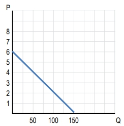
So now let's see how elasticity changes along a linear demand curve. A lot of students mix this up and tend to think that slope and elasticity are the same thing. Although they are slightly related, they are not the same, right? Slope is a ratio of changes between two variables where we're in a certain unit, but elasticity is a ratio of percentage changes, right? We've got percentage changes, and that little word "percentages" there makes a huge difference between the two definitions. So let's go over to this purple box where I can maybe show you an example of what's happening. When we have a price of $1 and we increase it to $2, what was our unit change in that situation? Well, we went from 1 to 2; we increased by 1, right? We increased by $1 there. But what was our percentage change? We started at 1 - whoa, calm down. Okay, we started at 1, and now we're at 2. We doubled our value, right? We started at 1 and doubled it up to 2. So our percentage change in that situation was 100%. We increased it 100% from 1 to 2. And how about this second situation? We were at a price of 2, and now we increased it to 3. Again, we have a unit change of 1, right? We just increased it by $1 there, but what about our percentage change this time? It's not 100 percent, right? We didn't double it again. We actually only increased it by half of the amount. We went from 2 to 3, we only increased it by 1, which is half of 2. In that situation, our percentage change was just 50% right, and that's because the numbers got bigger, right? So you could imagine from 3 to 4; we're still going to have a unit change of 1 but a smaller percentage change. 4 to 5, the percentage change is even smaller. So you're going to see that even though the change is linear, right, we have this constant change of 1 unit at a time, we're having different percentage changes every time, right? So even if you don't get everything on a really deep level there, just at least understand that we do have a difference here between slope and elasticity. Cool? So let's go ahead and go on to this graph where we've got a linear demand curve, and I just want to cut to the chase real quick. When we've got a linear demand curve, we're going to have sections of the line that are elastic, sections of the line that are inelastic, and a point on the line that's going to be unit elastic, alright? And that unit elastic point is going to be the point where we want to produce, and it's the point where revenue is maximized, okay? So I'm just going to cut through all the crap here and go straight to it. So right here, this section here to the left of the middle, right? So when you connect your demand curve from one axis to the other, like we have here, it's touching the price axis, and it's touching the quantity axis; you just go to the middle point, right? Right here is the middle, and you can visualize that very easily. Where's the middle of that line? Right there. So to the left of that middle point, which in the middle I'm going to highlight in green, right, to the left of that middle point, we are going to have elastic demand, and to the right of that point. What do you guys think? Yep. I heard someone. It's inelastic on that side of the point. Now here's the real kicker. Do you guys think at that specific point, what are we dealing with? Yep. Unit elastic is at that point right in the middle, and at that unit elastic point, just like I said, that's where we wanna produce, and that's where revenue is maximized. So let's go ahead and go to this table right here, where we've got the prices and quantities demanded, which are shown on that line on the graph. Okay? So I've gone ahead and taken these points and plotted them on the graph right there. Let's go ahead and calculate our total revenue in each of these cases. So total revenue, remember, is just price times quantity. So all we got to do is just multiply across here. So price times quantity, 0. 7 times 2, 14. It looks like we're doing our multiplication tables here again, so you could journey back to arithmetic, but let's go ahead and fill out this table. 34 times 8. 32. Right. So I'm just multiplying across price times quantity, and there we go. We've got all our total revenues. So you'll notice what's happening, right? We started with a revenue of 0 when we had a price of 8 and no quantity demanded. And as we lowered the price and people started to demand quanti...
- 0. Basic Principles of Economics1h 5m
- Introduction to Economics3m
- People Are Rational2m
- People Respond to Incentives1m
- Scarcity and Choice2m
- Marginal Analysis9m
- Allocative Efficiency, Productive Efficiency, and Equality7m
- Positive and Normative Analysis7m
- Microeconomics vs. Macroeconomics2m
- Factors of Production5m
- Circular Flow Diagram5m
- Graphing Review10m
- Percentage and Decimal Review4m
- Fractions Review2m
- 1. Reading and Understanding Graphs59m
- 2. Introductory Economic Models1h 10m
- 3. The Market Forces of Supply and Demand2h 26m
- Competitive Markets10m
- The Demand Curve13m
- Shifts in the Demand Curve24m
- Movement Along a Demand Curve5m
- The Supply Curve9m
- Shifts in the Supply Curve22m
- Movement Along a Supply Curve3m
- Market Equilibrium8m
- Using the Supply and Demand Curves to Find Equilibrium3m
- Effects of Surplus3m
- Effects of Shortage2m
- Supply and Demand: Quantitative Analysis40m
- 4. Elasticity2h 16m
- Percentage Change and Price Elasticity of Demand10m
- Elasticity and the Midpoint Method20m
- Price Elasticity of Demand on a Graph11m
- Determinants of Price Elasticity of Demand6m
- Total Revenue Test13m
- Total Revenue Along a Linear Demand Curve14m
- Income Elasticity of Demand23m
- Cross-Price Elasticity of Demand11m
- Price Elasticity of Supply12m
- Price Elasticity of Supply on a Graph3m
- Elasticity Summary9m
- 5. Consumer and Producer Surplus; Price Ceilings and Floors3h 45m
- Consumer Surplus and Willingness to Pay38m
- Producer Surplus and Willingness to Sell26m
- Economic Surplus and Efficiency18m
- Quantitative Analysis of Consumer and Producer Surplus at Equilibrium28m
- Price Ceilings, Price Floors, and Black Markets38m
- Quantitative Analysis of Price Ceilings and Price Floors: Finding Points20m
- Quantitative Analysis of Price Ceilings and Price Floors: Finding Areas54m
- 6. Introduction to Taxes and Subsidies1h 46m
- 7. Externalities1h 12m
- 8. The Types of Goods1h 13m
- 9. International Trade1h 16m
- 10. The Costs of Production2h 35m
- 11. Perfect Competition2h 23m
- Introduction to the Four Market Models2m
- Characteristics of Perfect Competition6m
- Revenue in Perfect Competition14m
- Perfect Competition Profit on the Graph20m
- Short Run Shutdown Decision33m
- Long Run Entry and Exit Decision18m
- Individual Supply Curve in the Short Run and Long Run6m
- Market Supply Curve in the Short Run and Long Run9m
- Long Run Equilibrium12m
- Perfect Competition and Efficiency15m
- Four Market Model Summary: Perfect Competition5m
- 12. Monopoly2h 13m
- Characteristics of Monopoly21m
- Monopoly Revenue12m
- Monopoly Profit on the Graph16m
- Monopoly Efficiency and Deadweight Loss20m
- Price Discrimination22m
- Antitrust Laws and Government Regulation of Monopolies11m
- Mergers and the Herfindahl-Hirschman Index (HHI)17m
- Four Firm Concentration Ratio6m
- Four Market Model Summary: Monopoly4m
- 13. Monopolistic Competition1h 9m
- 14. Oligopoly1h 26m
- 15. Markets for the Factors of Production1h 33m
- The Production Function and Marginal Revenue Product16m
- Demand for Labor in Perfect Competition7m
- Shifts in Labor Demand13m
- Supply of Labor in Perfect Competition7m
- Shifts in Labor Supply5m
- Differences in Wages6m
- Discrimination6m
- Other Factors of Production: Land and Capital5m
- Unions6m
- Monopsony11m
- Bilateral Monopoly5m
- 16. Income Inequality and Poverty35m
- 17. Asymmetric Information, Voting, and Public Choice39m
- 18. Consumer Choice and Behavioral Economics1h 16m
Total Revenue Along a Linear Demand Curve - Online Tutor, Practice Problems & Exam Prep
Understanding elasticity along a linear demand curve is crucial. Elasticity measures percentage changes, while slope measures unit changes. In a linear demand curve, demand is elastic to the left of the midpoint, inelastic to the right, and unit elastic at the midpoint, where total revenue is maximized. Total revenue, calculated as price times quantity, initially increases with demand until it reaches this unit elastic point, after which it declines. Recognizing these relationships helps in analyzing market behavior and optimizing revenue strategies.
Elasticity changes along a linear demand curve!
Total Revenue Along a Linear Demand Curve
Video transcript
What is the elasticity of demand when the price of the good changes from $3 to $5?
At what price is the elasticity of demand for the product equal to one?
At what price is revenue maximized?
Here’s what students ask on this topic:
What is the difference between slope and elasticity in a linear demand curve?
The slope of a linear demand curve measures the ratio of changes between two variables in specific units, such as dollars or quantity. In contrast, elasticity measures the ratio of percentage changes between these variables. For example, if the price increases from $1 to $2, the unit change is $1, but the percentage change is 100%. Elasticity provides a more nuanced understanding of how quantity demanded responds to price changes, as it accounts for the relative size of the changes. This distinction is crucial for analyzing market behavior and optimizing revenue strategies.
How does total revenue change along a linear demand curve?
Total revenue, calculated as price times quantity, changes along a linear demand curve in a predictable pattern. Initially, as the price decreases and quantity demanded increases, total revenue rises. This continues until it reaches a maximum point at the unit elastic point, which is the midpoint of the demand curve. Beyond this point, further decreases in price lead to a smaller increase in quantity demanded, causing total revenue to decline. Understanding this relationship helps in identifying the optimal price point for maximizing revenue.
What is the significance of the unit elastic point on a linear demand curve?
The unit elastic point on a linear demand curve is significant because it represents the price and quantity combination where total revenue is maximized. At this point, the percentage change in quantity demanded is exactly equal to the percentage change in price, resulting in no net change in total revenue. This point is located at the midpoint of the demand curve. Recognizing this point is crucial for businesses aiming to optimize their pricing strategies to maximize revenue.
How do you determine if a section of a linear demand curve is elastic or inelastic?
To determine if a section of a linear demand curve is elastic or inelastic, locate the midpoint of the curve. The demand is elastic to the left of this midpoint, meaning that the percentage change in quantity demanded is greater than the percentage change in price. To the right of the midpoint, the demand is inelastic, indicating that the percentage change in quantity demanded is less than the percentage change in price. At the midpoint, the demand is unit elastic, where the percentage changes in price and quantity demanded are equal.
Why is understanding elasticity important for revenue optimization?
Understanding elasticity is crucial for revenue optimization because it helps businesses determine how changes in price will affect total revenue. In the elastic region of the demand curve, lowering prices can increase total revenue, as the increase in quantity demanded outweighs the decrease in price. Conversely, in the inelastic region, raising prices can increase total revenue, as the decrease in quantity demanded is proportionally smaller than the increase in price. Identifying the unit elastic point, where total revenue is maximized, allows businesses to set optimal pricing strategies.