When exploring polar equations, four primary shapes frequently arise: the cardioid, limacon, rose, and lemniscate. Each of these shapes is characterized by specific equations that include variables such as r, θ, and trigonometric functions.
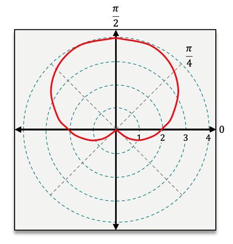
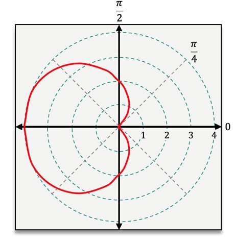
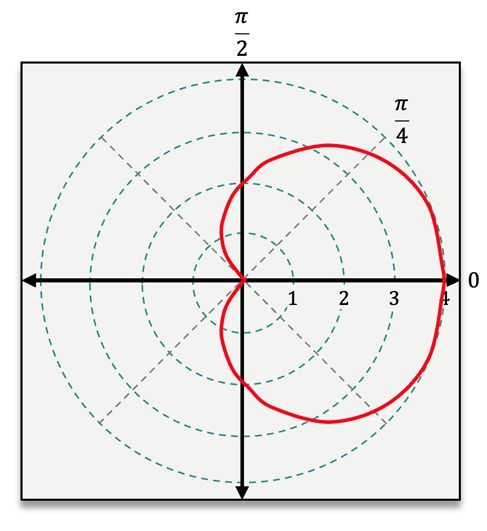
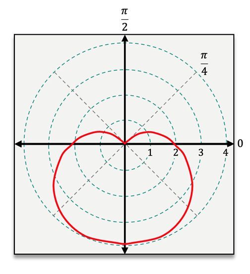
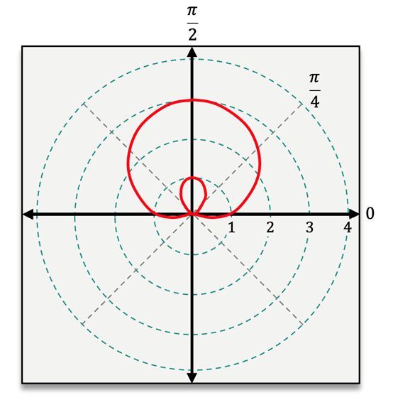
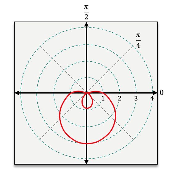
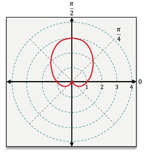
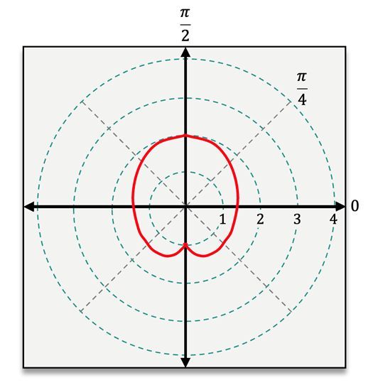
The cardioid resembles a heart shape and is defined by the equations r = a ± b cos(θ) or r = a ± b sin(θ), where both a and b are positive and equal (i.e., a = b). In contrast, the limacon shares the same equation form but allows for a to be either greater than or less than b. If a > b, the limacon has a dimple; if a < b, it features an inner loop.
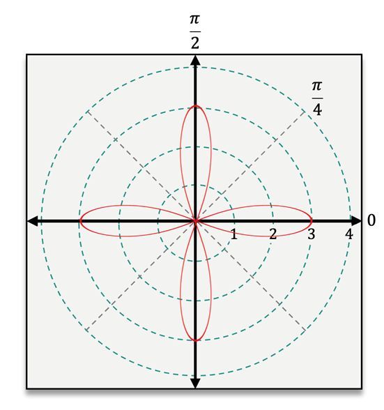
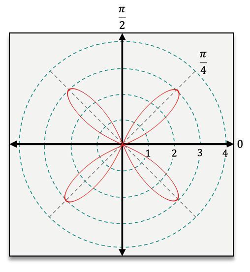
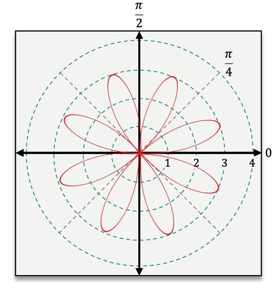
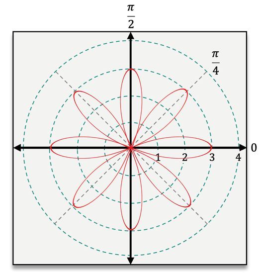
The rose curve, which resembles a flower, is represented by the equations r = a cos(nθ) or r = a sin(nθ). Here, a must be non-zero, and n is an integer greater than or equal to 2, indicating the number of petals. For example, if n = 4, the rose will have four petals.
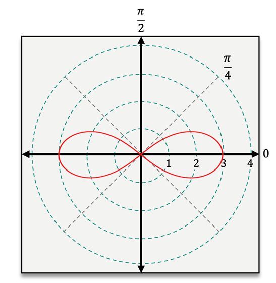
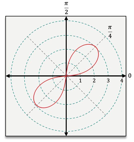
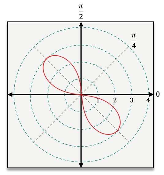
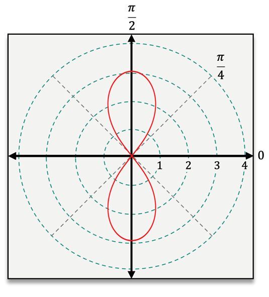
Lastly, the lemniscate, which looks like an infinity symbol, is defined by the equations r² = ±a² cos(2θ) or r² = ±a² sin(2θ). This shape is unique in that it includes r², making it easily identifiable among polar equations.
To classify these shapes, consider the structure of the equation. For instance, the equation r = 1 + cos(θ) indicates a cardioid since it contains addition and a = b = 1. Conversely, the equation r = 4 sin(2θ) suggests a rose because it has the form r = a sin(nθ) with n = 2, and it does not include r².
Understanding these equations and their characteristics is essential for graphing polar shapes accurately. By recognizing the forms and parameters, one can predict the appearance of the graph associated with each equation.