In exploring the graph of the tangent function, it's essential to understand its relationship with sine and cosine. The tangent of an angle can be expressed as the ratio of sine to cosine, represented mathematically as:
\[ \tan(x) = \frac{\sin(x)}{\cos(x)} \]
Starting from the origin (0,0), we can evaluate the tangent function at key points. At \(x = 0\), the tangent value is:
\[ \tan(0) = \frac{\sin(0)}{\cos(0)} = \frac{0}{1} = 0 \]
Moving to \(x = \frac{\pi}{4}\), we find:
\[ \tan\left(\frac{\pi}{4}\right) = \frac{\sin\left(\frac{\pi}{4}\right)}{\cos\left(\frac{\pi}{4}\right)} = \frac{\frac{\sqrt{2}}{2}}{\frac{\sqrt{2}}{2}} = 1 \]
Conversely, at \(x = -\frac{\pi}{4}\), the tangent value is:
\[ \tan\left(-\frac{\pi}{4}\right) = \frac{\sin\left(-\frac{\pi}{4}\right)}{\cos\left(-\frac{\pi}{4}\right)} = \frac{-\frac{\sqrt{2}}{2}}{\frac{\sqrt{2}}{2}} = -1 \]
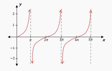
At \(x = \frac{\pi}{2}\) and \(x = -\frac{\pi}{2}\), the tangent function becomes undefined due to division by zero, leading to vertical asymptotes at these points. The asymptotes for the tangent function occur at odd multiples of \(\frac{\pi}{2}\), specifically at:
\[ x = \frac{\pi}{2} + n\pi \quad (n \in \mathbb{Z}) \]
This results in asymptotes at \(x = -\frac{3\pi}{2}, -\frac{\pi}{2}, \frac{\pi}{2}, \frac{3\pi}{2}\), indicating that the function approaches infinity at these points. The graph of the tangent function exhibits a repeating pattern every \(\pi\) units, distinguishing it from the secant function, which has a period of \(2\pi\).
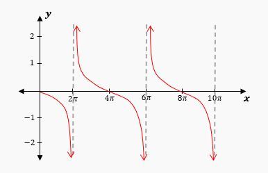
The period of the tangent function can be calculated using the formula:
\[ \text{Period} = \frac{\pi}{b} \]
where \(b\) is the coefficient of \(x\) in the function. For example, in the function \(y = \tan\left(\frac{\pi}{2}x\right)\), the period is:
\[ \text{Period} = \frac{\pi}{\frac{\pi}{2}} = 2 \]
This means the tangent function will repeat its pattern every 2 units along the x-axis. To graph this function, one would plot the asymptotes at \(x = -1\) and \(x = 1\), and then sketch the curve that rises from the left asymptote to the right asymptote, repeating this pattern every 2 units.
Understanding these properties of the tangent function allows for effective graphing and analysis, reinforcing the connections between trigonometric functions and their graphical representations.