Transformations of functions are essential concepts in mathematics that involve manipulating a function to change its position or shape. There are three primary types of transformations: reflections, shifts, and stretches. Understanding these transformations can simplify the study of functions significantly.
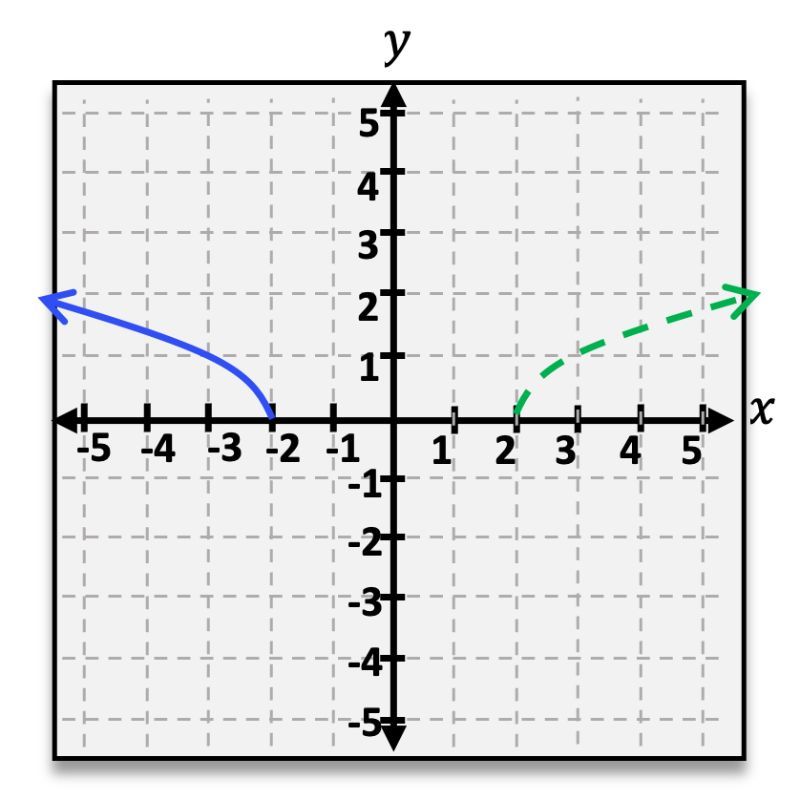
A reflection occurs when a function is flipped over a specific axis. For instance, reflecting a function over the x-axis changes its output to the negative of the original function, represented mathematically as f(x) → -f(x). This transformation effectively "folds" the graph over the axis.
A shift involves moving a function horizontally or vertically. The general form for a shift is f(x) → f(x - h) + k, where h indicates the horizontal shift and k represents the vertical shift. For example, if a function is shifted right by 3 units and up by 2 units, it would be expressed as f(x - 3) + 2.
A stretch transformation occurs when a function is vertically stretched or compressed. This is represented as f(x) → c * f(x), where c is a constant. If c is greater than 1, the function is stretched; if c is between 0 and 1, the function is compressed.
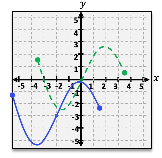
To illustrate these transformations, consider the function f(x) = |x|. If we analyze the transformations of this function, we can match various transformed functions to their corresponding graphs. For example, the function p(x) = |x - 3| + 2 represents a shift transformation, moving the graph to the right by 3 units and up by 2 units. The function q(x) = -|x| represents a reflection over the x-axis, flipping the graph upside down. Lastly, a function like r(x) = -2|x| combines both a reflection and a vertical stretch, as indicated by the negative sign and the constant factor of 2.
In summary, understanding these basic transformations—reflections, shifts, and stretches—enables students to analyze and manipulate functions effectively. Recognizing how these transformations affect the function's graph is crucial for mastering more complex mathematical concepts.