In the study of gravitational forces, particularly for non-spherical mass distributions, we utilize calculus to derive the gravitational force acting on a mass due to a distribution of mass. According to Newton's law of gravity, the gravitational force \( F \) between two point masses \( m_1 \) and \( m_2 \) separated by a distance \( r \) is given by the equation:
\( F = \frac{G m_1 m_2}{r^2} \)
For spherical objects, we can simplify the problem by treating the mass as concentrated at a point, specifically at the center of mass. However, when dealing with non-spherical distributions, this simplification is no longer valid. Instead, we can break the mass into infinitesimally small pieces, referred to as differential mass elements \( dm \). Each of these elements can be treated as a point mass, generating a tiny gravitational force \( dF \) on another mass \( m \) located at a distance \( r \) from the mass element.
The expression for the differential force \( dF \) due to a differential mass \( dm \) is given by:
\( dF = \frac{G \, dm \, m}{r^2} \)
To find the total gravitational force \( F \), we need to integrate \( dF \) over the entire mass distribution:
\( F = \int dF = G m \int \frac{dm}{r^2} \)
In this integral, \( G \) and \( m \) can be factored out as constants since they do not change during the integration process. The next step involves determining the expression for \( r \) based on the geometry of the mass distribution. For example, if we consider a hollow ring, we can use the Pythagorean theorem to express \( r \) as:
\( r = \sqrt{R^2 + d^2} \)
where \( R \) is the radius of the ring and \( d \) is the distance from the center of the ring to the mass \( m \).
Next, we decompose the total force into its x and y components. Due to symmetry, the y-components of the forces from opposite sides of the ring will cancel each other out, leaving only the x-components contributing to the total force. The x-component of the differential force can be expressed as:
\( dF_x = dF \cos(\theta) \)
Using the relationship of the triangle formed by the geometry, we can express \( \cos(\theta) \) in terms of the sides of the triangle, leading to:
\( dF_x = \frac{G m}{r^2} \cdot \frac{d}{r} \)
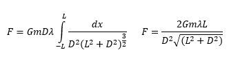
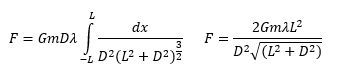
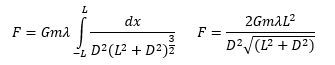
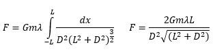
Substituting the expression for \( r \) into the equation, we can simplify the integral further. After pulling out constants from the integral, we arrive at:
\( F = \frac{G M d}{(R^2 + d^2)^{3/2}} \int dm \)
Since the integral of \( dm \) over the entire mass distribution equals the total mass \( M \), we finally obtain the expression for the gravitational force:
\( F = \frac{G M^2 d}{(R^2 + d^2)^{3/2}} \)
This formula allows us to calculate the gravitational force exerted by a non-spherical mass distribution, such as a hollow ring, on a point mass located at a distance \( d \) from the center of the ring.