Hey everyone. So at this point in the course, we should be very familiar with the sine and cosine trigonometric functions, and we've recently talked about how these trig functions will relate to the unit circle. Now what we're going to be talking about in this video is how you can take the sine and cosine functions, and graph them on a standard xy graph. This might sound a bit intimidating since we don't know at all what these graphs are going to look like, but don't sweat it because it turns out that using the values that we're familiar with on the unit circle, we can actually graph these in a very straightforward way using these values. So without further ado, let's get right into things.
Now I want you to recall how the sine is associated with the y coordinates when you look at a unit circle, and the cosine is associated with the x coordinates. You'll see that these values will repeat as you go around the unit circle. For example, if we're looking at the sine, we can see that our sine value starts at 0, then it goes to 1, then to 0, then to negative one, and then it starts repeating. So it goes back to 0, then to 1, then 0, and it just repeats as you go around.
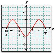
You'll notice for the sine and cosine, these values repeat around the unit circle. And because of this, you're going to see some interesting behavior in their graphs. Let's say we're looking at the sine graph where y=sinx. We can figure out what this graph looks like by plotting some points. For the sine of 0, based on our unit circle, the sine of 0 is just going to be 0. Now, for the sine of π2, according to our unit circle, it is 1. For the sine of π, the sine of π is 0. If we go to 3π2, the sine of 3π2 is negative 1. So the sine of 2π would be a full trip around the circle right back to 0, and then the sine of 5π2 would be a full trip around the circle, and then all the way back up to 1, meaning that your graph is going to look something like this. If I go ahead and connect these points with the smooth curve, you'll notice something kind of interesting happens in our graph.
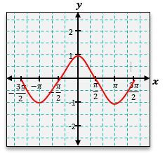
We get this kind of wave that shows up, and that's what happens when you have these repeating values. So both the sine and cosine are going to be graphs that look like waves. Now, to prove this to ourselves, let's take a look at the cosine graph as well. The cosine is going to be associated with the x coordinates, and when we look at the cosine of 0, we can see that it starts right here at 1. For the cosine of π2, it's going to be at 0. For the cosine of π, that's going to be at negative one. For the cosine of 3π2, it's going to be back at 0, and then you can keep plotting these points. So for 2π, we're going to be back up at 1. And then for the cosine of 5π2, we're going to be back at 0, meaning your graph is going to look something like this. Notice how we get the same kind of wave pattern that we got for the sine, except this graph starts a bit differently.
Notice how our graph starts at an output of 1 for the cosine, and our graph starts at an output of 0 for the sine. But if you look at the unit circle, this should make perfect sense because we can see at 0 radians, our cosine starts at 1 and our sine starts at 0. So that's why we have the graphs that look like this and then show this waving pattern based on the repeating values that we saw. Now some other terminology you should be familiar with are the high points and low points of our wave. The high points are known as crests, or they're also called peaks.
So the peaks of the wave are going to be all these places that we see our high values at, our highest values on the wave. And another thing you should be familiar with is the low points, which are known as troughs or valleys. The valleys are going to be these lowest points on each of the waves. Now it turns out these peaks and valleys are not always going to be a positive one and negative one for the sine and cosine. Because recall that we learned back in algebra that you can actually have transformations on your function, and it turns out that the sine and cosine graphs can also go through transformations.
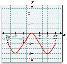
Now one of the simplest transformations we learned about was something called the vertical shift. And this occurs when you go ahead and take a function and add some constant k to it, which will cause it to vertically shift up or down. Well, it turns out for these sine and cosine graphs, you could also add a constant k, which vertically shifts the function. So adding a constant to the sine or cosine will shift the wave up or down in a certain way. Now if the k value that you have is positive, the graph is going to shift up, whereas if the k value is negative, the graph will shift down.
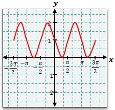
Now to understand this a bit better, let's actually try an example where we put both these concepts together. So here we have a situation where we are asked to graph the function y=sinx+1. Notice we have a sine function we're dealing with, and it's been shifted in some kind of way. Now to solve this problem, what I'm first going to do is try graphing the function y=sinx. So I'm gonna go ahead and ignore this plus one for now.
Now recall for the sine of x, we start at a value of 0, at an output of 0, and then we reach a peak at π2, then we go back to 0 through π, and then we reach a valley at 3π2, then we go back to 0 over 2π, and we reach another peak at 5π2. But how exactly could we graph the function y=sinx+1? Well, this is what we're ultimately looking for in this problem, and because we have a plus one, this tells us that we're gonna have some kind of vertical shift. It's a positive number, meaning it's going to shift up. So all we need to do is take this entire graph and shift it up by 1.
So this point is going to be at an output of 1. This peak would be at an output of 2, and then this point would be at an output of 1, and then this valley at negative one would now be at an output of 0. So what we're going to do is trace a curve that looks like this. We'll have a peak at an output of 2, then we'll go down to 1, and then we'll reach our valley at an output of 0, then we'll go back up to an output of 1, and then we'll reach a peak at an output of 2. So this would be the graph for y=sinx+1, and that is the answer to this example.
Hopefully, this gave you a good understanding of how to graph sine and cosine functions and deal with any kind of vertical shifts if you have them. I hope you found this video helpful. Thanks for watching.