1. Limits and Continuity
Introduction to Limits
Problem 35a
Textbook Question
Postage rates Assume postage for sending a first-class letter in the United States is $0.47 for the first ounce (up to and including 1 oz) plus $0.21 for each additional ounce (up to and including each additional ounce).
a. Graph the function p=f(w) that gives the postage p for sending a letter that weighs w ounces, for 0<w≤3.5.
 Verified step by step guidance
1
Step 1: Understand the problem. We need to graph the function p = f(w) that represents the postage cost p for a letter weighing w ounces, where 0 < w ≤ 3.5. The cost is $0.47 for the first ounce and $0.21 for each additional ounce.
Step 2: Define the function. For 0 < w ≤ 1, the cost is $0.47. For 1 < w ≤ 2, the cost is $0.47 + $0.21 = $0.68. For 2 < w ≤ 3, the cost is $0.68 + $0.21 = $0.89. For 3 < w ≤ 3.5, the cost is $0.89 + $0.21 = $1.10.
Step 3: Identify the type of function. This is a piecewise function, where each piece is constant over the intervals (0, 1], (1, 2], (2, 3], and (3, 3.5].
Step 4: Plot the graph. On the x-axis, represent the weight w in ounces, and on the y-axis, represent the postage cost p in dollars. Plot horizontal line segments for each interval: from (0, 1] at $0.47, from (1, 2] at $0.68, from (2, 3] at $0.89, and from (3, 3.5] at $1.10.
Step 5: Indicate the endpoints. Use closed circles at the right endpoints of each interval to indicate that the value is included, and open circles at the left endpoints (except for the first interval) to indicate that the value is not included.
Verified video answer for a similar problem:This video solution was recommended by our tutors as helpful for the problem above
Video duration:
5mWas this helpful?
Key Concepts
Here are the essential concepts you must grasp in order to answer the question correctly.
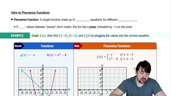
Piecewise Functions
A piecewise function is defined by different expressions based on the input value. In this case, the postage function p=f(w) changes depending on the weight w of the letter. For weights up to 1 ounce, the cost is a flat rate, while for weights above 1 ounce, an additional charge applies for each extra ounce. Understanding how to construct and graph piecewise functions is essential for accurately representing the postage rates.
Recommended video:
 05:36
05:36Piecewise Functions
Graphing Functions
Graphing functions involves plotting points on a coordinate system to visually represent the relationship between variables. For the postage function, the x-axis represents the weight of the letter (w), and the y-axis represents the postage cost (p). Knowing how to plot points and connect them appropriately, especially for piecewise functions, is crucial for creating an accurate graph that reflects the postage rates.
Recommended video:
 5:53
5:53Graph of Sine and Cosine Function
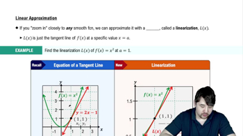
Linear Functions
Linear functions are mathematical expressions that create straight lines when graphed. In the context of the postage rates, the cost for each additional ounce after the first is a linear increase of $0.21 per ounce. Recognizing the linear nature of the additional charges helps in understanding how to calculate the total postage for weights greater than 1 ounce and aids in graphing the function correctly.
Recommended video:
 07:17
07:17Linearization
 6:47m
6:47mWatch next
Master Finding Limits Numerically and Graphically with a bite sized video explanation from Callie
Start learning