4. Applications of Derivatives
Differentials
Problem 30
Textbook Question
21–32. Mean Value Theorem Consider the following functions on the given interval [a, b].
a. Determine whether the Mean Value Theorem applies to the following functions on the given interval [a, b].
b. If so, find the point(s) that are guaranteed to exist by the Mean Value Theorem.
ƒ(x) = x + 1/x; [1,3]
 Verified step by step guidance
1
Step 1: Verify the conditions for the Mean Value Theorem (MVT). The function must be continuous on the closed interval [a, b] and differentiable on the open interval (a, b). For the function f(x) = x + 1/x, check continuity and differentiability on [1, 3].
Step 2: Check continuity. The function f(x) = x + 1/x is continuous on [1, 3] because it is composed of continuous functions (a polynomial and a reciprocal function) and x is never zero in this interval.
Step 3: Check differentiability. The function f(x) = x + 1/x is differentiable on (1, 3) because both x and 1/x are differentiable for x > 0, and there are no points of discontinuity or non-differentiability in (1, 3).
Step 4: Since f(x) is continuous on [1, 3] and differentiable on (1, 3), the Mean Value Theorem applies. According to the MVT, there exists at least one c in (1, 3) such that f'(c) = (f(b) - f(a)) / (b - a).
Step 5: Calculate f'(x) and solve f'(c) = (f(3) - f(1)) / (3 - 1) to find the value of c. First, find f'(x) by differentiating f(x) = x + 1/x, which gives f'(x) = 1 - 1/x^2. Then, solve 1 - 1/c^2 = (f(3) - f(1)) / 2 to find the value of c.
Verified video answer for a similar problem:This video solution was recommended by our tutors as helpful for the problem above
Video duration:
7mWas this helpful?
Key Concepts
Here are the essential concepts you must grasp in order to answer the question correctly.
Mean Value Theorem
The Mean Value Theorem (MVT) states that if a function is continuous on a closed interval [a, b] and differentiable on the open interval (a, b), then there exists at least one point c in (a, b) such that the derivative at that point equals the average rate of change of the function over the interval. This theorem is fundamental in understanding the behavior of functions and their derivatives.
Recommended video:

 06:11
06:11Fundamental Theorem of Calculus Part 1
Continuity and Differentiability
For the Mean Value Theorem to apply, the function must be continuous on the closed interval [a, b] and differentiable on the open interval (a, b). Continuity ensures that there are no breaks or jumps in the function, while differentiability means that the function has a defined slope (derivative) at every point in the interval, which is crucial for finding the point c where the MVT holds.
Recommended video:
 05:34
05:34Intro to Continuity
Finding the Derivative
To apply the Mean Value Theorem, one must first find the derivative of the function. The derivative provides the instantaneous rate of change of the function at any point. In this case, for the function ƒ(x) = x + 1/x, calculating the derivative will help identify the point(s) c where the derivative equals the average rate of change over the interval [1, 3], which is necessary for fulfilling the conditions of the MVT.
Recommended video:
 06:02
06:02The Second Derivative Test: Finding Local Extrema