0. Functions
Piecewise Functions
Problem 30
Textbook Question
Graphing functions Sketch a graph of each function.
ƒ(x) = { 2x if x ≤ 1 , 3-x if x > 1
 Verified step by step guidance
1
Identify the type of function: This is a piecewise function, which means it is defined by different expressions depending on the value of x.
Determine the domain for each piece: The function is defined as f(x) = 2x for x ≤ 1 and f(x) = 3 - x for x > 1.
Sketch the first piece: For f(x) = 2x when x ≤ 1, this is a linear function with a slope of 2. Plot the line starting from x = -∞ to x = 1, including the point (1, 2) as a solid dot since x = 1 is included.
Sketch the second piece: For f(x) = 3 - x when x > 1, this is also a linear function with a slope of -1. Plot the line starting just after x = 1, with an open circle at (1, 2) since x = 1 is not included in this piece, and continue to x = ∞.
Combine the pieces: Ensure the graph is continuous at x = 1 by checking the values of both pieces at this point. The first piece ends at (1, 2) and the second piece starts just after (1, 2), so the graph is not continuous at x = 1.
Verified video answer for a similar problem:This video solution was recommended by our tutors as helpful for the problem above
Video duration:
6mWas this helpful?
Key Concepts
Here are the essential concepts you must grasp in order to answer the question correctly.
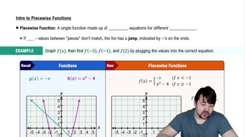
Piecewise Functions
A piecewise function is defined by different expressions based on the input value. In this case, the function ƒ(x) has two distinct rules: 2x for x values less than or equal to 1, and 3-x for x values greater than 1. Understanding how to evaluate and graph each piece separately is crucial for accurately representing the overall function.
Recommended video:
 05:36
05:36Piecewise Functions
Graphing Techniques
Graphing techniques involve plotting points and understanding the behavior of functions across their domains. For piecewise functions, it is important to identify the points where the function changes its rule, and to ensure continuity or discontinuity at those points. This includes determining the endpoints and whether they are included in the graph.
Recommended video:
 06:15
06:15Graphing The Derivative
Continuity and Discontinuity
Continuity refers to a function being unbroken at a point, meaning the function's value at that point matches the limit as it approaches from either side. In the case of the given piecewise function, checking continuity at x = 1 is essential, as it determines whether the graph has a jump or is smooth at that transition point.
Recommended video:
 05:34
05:34Intro to Continuity

Related Videos
Related Practice