Understanding how to find the area underneath a curve is a fundamental concept in calculus, particularly when dealing with functions that do not form simple geometric shapes like triangles or squares. To estimate this area, we can use a method that involves dividing the area under the curve into smaller, manageable sections, typically rectangles.
The first step in this process is to determine the number of rectangles, denoted as n, which also represents the number of subintervals. By breaking the curve into these rectangles, we can approximate the area by summing the areas of each rectangle. The area of a rectangle is calculated using the formula:
Area = Width × Height
In this context, the width of each rectangle is referred to as Δx, which can be calculated using the formula:
Δx = (b - a) / n
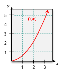
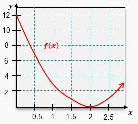
Here, a and b are the lower and upper bounds of the interval over which we are calculating the area. For example, if we are estimating the area under a curve from x = 0 to x = 2 using four rectangles, we would calculate:
Δx = (2 - 0) / 4 = 0.5
Next, to find the height of each rectangle, we evaluate the function at specific points known as the left endpoints of each rectangle. For instance, if we have four rectangles, we would evaluate the function at f(0), f(0.5), f(1), and f(1.5). The heights of the rectangles are then determined by these function values.
Once we have the width and heights, we can compute the total area under the curve by summing the areas of all rectangles:
Total Area ≈ Δx × (f(0) + f(0.5) + f(1) + f(1.5))
As we increase the number of rectangles, the approximation becomes more accurate. For example, using two rectangles might yield an area of 7, while using four rectangles could give an area of 6.25. The more rectangles we use, the closer our estimate will be to the actual area under the curve, as the rectangles will better conform to the shape of the curve, reducing the area that extends beyond the curve.
In summary, estimating the area under a curve involves dividing the area into rectangles, calculating their widths and heights based on the function values, and summing their areas. This method provides a practical approach to approximating areas that cannot be easily calculated using standard geometric formulas.