Graphing Rational Functions - Online Tutor, Practice Problems & Exam Prep

Understanding rational functions involves identifying key components such as vertical and horizontal asymptotes, x and y intercepts, and the behavior of the graph around these points. Transformations like shifts and reflections can modify the basic graph of $(1/x)$. The domain is determined by the denominator, while intercepts and asymptotes guide the overall shape. Analyzing intervals between these components helps in sketching the graph accurately, ensuring a comprehensive understanding of rational functions.

Graphing Rational Functions Using Transformations

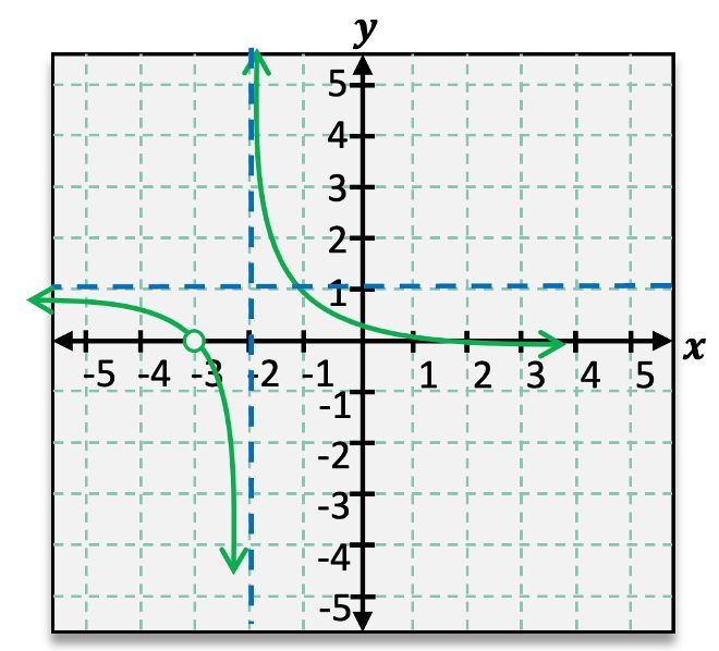
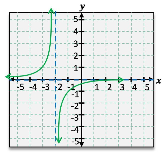
Hey, everyone. We now know all of the components of the graph of a rational function. But taking those components and putting them all together to form an actual graph can be the hardest part. So here, we're going to take the most basic of rational functions, 1x, and simply apply rules of transformations to it in order to graph a more complicated rational function. So here, I'm going to walk you through using transformations to graph this function without doing a single calculation. We're just going to take our function 1x and pick it up and move it around a little bit to get the graph of our new function, which will end up looking something like this. So let's go ahead and walk through how to get there.

Now, with our function g(x) here, we see that it looks really similar to 1x. We even have this 1x here. We just have these extra numbers added in. Now these numbers represent transformations to our function. And when working with rational functions, we're going to focus on two types of transformations in particular, reflections and shifts, because they are the most commonly occurring transformations when working with rational functions.

Now remember, whenever we have a negative outside of our function, that tells us we're going to have a reflection over the x-axis, whereas having a negative inside of our function is a reflection over the y-axis. Now with h and k over here, x-h, h represents a horizontal shift side to side by some number h units. And then k represents a vertical shift up and down by some number k units. So let's go ahead and apply these transformations to our function here.

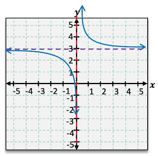
Now our function 1x, our graph here, we see that we have asymptotes at our x and y axes, and we also have these points on our graph at (1,1) and (-1,-1) that are going to serve as sort of reference or test points for us as we graph our new function. So we're going to focus on transforming our asymptotes and these points in order to get the graph of g(x) here. So let's go ahead and start with step 1, which is to find the vertical asymptote and plot it at x=h. Now looking at our function here, 1x-3+1, I have x-3, so h here is 3. I'm going to have a vertical asymptote at x=3. Now, we can go ahead and plot that on our graph using a dashed line because it is an asymptote.

Now we can go ahead and move on to step 2, which is to plot our horizontal asymptote at y=k. Now, looking back at our function here, I have this plus 1 on the end, so I know that k is going to be 1. I'm going to plot my horizontal asymptote at y=1, again, using a dashed line. Now, compared to our original asymptotes at our axes, we see that these got shifted h units over and k units up. And we see this transformation happening here. So let's keep transforming our graph.

Now moving on to step number 3, we want to go ahead and determine if there is a reflection. Now remember, our reflection is if we have these negatives that got put into our function. And looking at my function, I don't have any negatives that got added in there, So, I do not have a reflection. Now if I did, I would take those test points (1,1) and (-1,-1) and simply reflect them over x or y accordingly. But I don't need to do that here. So let's go ahead and move on to step 3b and go ahead and shift our test points by h,k. Now we know that h,k is just 3,1 because we already plotted those at our asymptotes. So I'm going to take my test points, (1,1), and (-1,-1), and shift them accordingly. So my first point here, I'm going to go ahead and shift that 3 units over to the right and then 1 unit up, landing me at the point (4,2). Then my other test point, which is right here at (-1,-1), I'm going to shift that again 3 units to the right and one unit up, landing me at (2,0).

So I've now shifted both my asymptotes and those reference points. So I can go ahead and move on to my final step here, which is going to be to sketch my curves approaching the asymptotes. So looking at this first point here, I'm going to approach that asymptote going up and then approach my horizontal asymptote this way. Then my other test point, same thing, approaching my asymptotes on either side.

And now I have the final graph of my function. Now these are my curves here. I'm going to highlight them just so you can see them a little bit better. And you'll notice that this looks almost the exact same as our graph of 1x. It's just picked up and moved over, just like I said. Now, we want to look at one other thing here, our domain and our range. Now, our domain and range are going to be split by our asymptotes. And we're going to write them in set notation using this union symbol, which just represents a union between two sets. Now our domain is actually always going to go from negative infinity until I reach my asymptote at 3 and then continue on from 3 to infinity. So looking at the graph I have here, I'm going to go from negative infinity until I reach that asymptote at 3. And then I have a break at that asymptote because my domain is not defined there. And I pick back up and go from 3 to infinity. Then for my range, the same exact thing is going to happen. We're going to go from negative infinity to k and then from k to infinity because k is where my asymptote is. So looking at my function here, I know I go from negative infinity until I reach that asymptote where my domain is not defined at 1, and then continuing on from 1 to infinity. Now you'll notice that these are enclosed in parentheses rather than square brackets because we know that these numbers are not included in our domain or range.

So now that we know how to graph using transformations, let's get some more practice.

Example 1

In this problem, we're asked to graph the given function as a transformation of 1/x2. And here, I have the function g(x)=-1(x-2)2. So let's go ahead and graph this, starting with step 1, which is to find our vertical asymptote and plot it at x=h. Now, looking at my function, knowing that this is a transformation of 1/x2, I want to go ahead and identify h, which, in this case, is just 2. So, I'm going to plot my vertical asymptote at x=2, using a dashed line.

Now, for step number 2, we want to plot our horizontal asymptote at y=k. In this case, I don't have a value for k; it's just 0 because it didn't get transformed. So y is simply 0 for my horizontal asymptote, and it's actually at the same exact place as the horizontal asymptote of my original function. So that didn't really get shifted.

Now, we want to move on to step 3 and identify if there is a reflection happening, which we can tell whether there is a negative outside or inside of our function. Here, my negative is right here, and it makes my entire function negative. So, I do have a reflection, and that reflection is over the x axis. So, I'm going to take these two test points or reference points that I have here, and I am going to go ahead and reflect them over the x axis accordingly. So, looking at my points, starting with 1, 1, remember, we can think of a reflection as folding it in half at the x axis and kind of stamping that point on the other side. So here 1, 1 will end up right here, and then -1, 1 will end up here, reflected over that x axis. Now, we want to go ahead and shift these points by h, k. And then h here is 2, k is simply 0. So, we're just going to shift these two points or two units over to the right. So, starting with my point at 1, -1 shifting that 2 over, it's going to end up right over here. And then my other point is going to get shifted 2 over. And it's actually going to end up exactly where my other point was, right here. So, I have my two new points that have been both reflected and shifted. And we can go ahead and move on to our final step and simply sketch our curves approaching our asymptotes.

So let's go ahead and do that here. Approaching my asymptote on either side, I know that the shape is the exact same as my original 1/x2, but we've just been reflected and shifted. So here's my new function. We have fully crafted. Let's go ahead and identify our domain and our range. Now, our domain is going to go from negative infinity until we reach our asymptote where it's going to stop and then continue on the other side of my asymptote. So from negative infinity to my asymptote here is negative infinity to 2 and then from 2 to infinity.

Now as for my range, because we're only on one side of our x axis here, we only go from negative infinity up until we reach that asymptote, which happens to be at the x axis. If we were up here, our range would be different. But since we're down here, it goes from negative infinity until 0, where that asymptote is.

Now that we've graphed with this transformation and identified our domain and our range, thanks for watching, and I'll see you in the next video.

Graph the rational function using transformations.

$f\left(x\right)=-\frac{1}{x}+3$

• A.
• B.
• C.
• D.

Graph the rational function using transformations.

$f\left(x\right)=\frac{1}{\left(x+3\right)^2}-2$

• A.
• B.
• C.
• D.

How to Graph Rational Functions

Hey everyone. We now know all of the components of the graph of a rational function, and we're not always going to be able to graph rational functions using basic transformations. Sometimes, like with this function here, there's going to be a little bit more going on. So we're going to take all of these components and put them together now in order to fully graph a rational function from scratch. It might feel like a lot, and that's okay. I'm going to walk you through it step by step. And if you follow these steps, you'll be able to graph any rational function. So let's go ahead and not waste any time and get into graphing.

Looking at my function here, I have 2x-3x-1. Starting with step number 1, we want to factor and find the domain. Looking at my function, it can't be factored any more than it already is, so we can just go ahead and skip straight to finding our domain by setting our denominator equal to 0. My denominator is x minus 1. Adding 1 to both sides here, I end up with x is equal to 1. Since this is my domain, I know that this is what my x value cannot be because it would make my denominator 0. So my domain is simply x such that x cannot be equal to 1.

Now we finished step 1. Let's move on to step 2 and go ahead and find any holes that may exist in our graph by setting our common factors equal to 0. Looking at my function, I again don't have any common factors here. So I don't have to worry about this step. And we can move on to step 2b and go ahead and put our function in lowest terms. Taking another look at our function, I can't cancel anything out because it already didn't have common factors. So I can go ahead and move on to step 3 and find my x intercepts.

To find my x intercepts, I'm going to set my numerator equal to 0, which is the equivalent of simply solving the equation f(x)=0. My numerator here, 2x-3, if I add 3 to both sides, it cancels, leaving me with 2x=3. And then to isolate x, I want to divide both sides by 2. That leaves me with x is equal to 32. Or if you want that as a decimal, this is also just 1.5. So I can go ahead and plot that on my graph at x equals 1.5.

But we also want to determine the behavior of our graph at this x intercept the same way we did with polynomials by looking at the multiplicity. Looking back at my original function, 2x-3x-1, 2x-3 is a factor that only occurs once, which tells us that our multiplicity is 1. Now because our multiplicity is 1, this is an odd number, so that tells me that my graph is fully going to cross the x-axis at that point, which I can denote here and then I can fix that later whenever I fully sketch my graph.

Okay, let's move on to our y-intercept in step 4 and compute f of 0 by plugging 0 into our function. Plugging 0 into my function here, I get 2×0-3, which gives me -3 over 0 minus 1, -1. Now, this simplifies to just positive 3, so my y-intercept is 3. And I can go ahead and plot that on my graph as well right on that y-axis.

Now that we have our intercepts, let's go ahead and move on to finding our asymptotes. So my first asymptote that I want to find is my vertical asymptote. And here, I'm just going to set my denominator equal to 0. Now, because we didn't have any common factors that canceled when we put our function in lowest terms, this is going to be the same thing as finding our domain. And we just have x minus 1 equals 0. So I can go ahead and add 1 to both sides, And I'm simply left with x is equal to 1 because that cancels, and that's all I'm left with. So let's go ahead and plot our vertical asymptote on our graph at x equals 1. I'm using a dash line because this is an asymptote.

Let's go ahead and move on to step 6 and find our horizontal asymptote. So here to find our horizontal asymptote, we're looking at the degrees of both the numerator and the denominator. And looking at my function here, 2x-3x-1, I have a degree of 1 in that numerator. I also have a degree of 1 in the denominator. So these degrees are equal to each other. Now because they're equal to each other, that tells me I need to divide my leading coefficients, and my leading coefficient in my numerator is simply 2. And then in my denominator, I have this 1 here. So taking those and dividing them 2 over 1 gives me a horizontal asymptote at y equals 2. So let's go ahead and plot that asymptote on our graph at y equals 2, again using a dash line because it is an asymptote.

Okay. Now that we have all of this information, we still don't know exactly what's happening all around these known components. So we're going to have to do something similar or the exact same that we did with polynomials and divide our graph up into intervals. Now our intervals with our rational function are going to be determined by our vertical asymptotes and our x intercepts. So we're still going to take a look at our graph from left to right. And along the way, we're going to look for those known components in order to break our graph into intervals and find the behavior within each of those intervals. So let's go ahead and go back up to our graph here in order to determine those intervals.

Starting on that left side, going until I reach my first known component, either a vertical asymptote or an x intercept, the first thing I reach is this vertical asymptote at x equals 1. So from negative infinity to that first known point at 1 is my first interval. Then my next interval starting from that one going until I reach the next known component, I have this x intercept almost right next to it. So my next interval is simply from 1 to 3/2, a really small interval, but an interval nonetheless. Now, finally, from 3/2 to infinity is my final interval here because there are no other known components.

Now that we have these intervals, we need to choose a value for x in each of them in order to plot a point to determine the behavior. So in this first interval, negative infinity to 1, remember you want to choose something that's in your graph so that you're actually able to plot it. So the first point I'm going to choose is x equals -2. Then from 1 to 1.25 (which is the same thing as 5/4), we don't have a ton of options here because this is such a tiny, tiny interval. So I'm going to choose 1.25. Now, for my final interval from 3/2 to infinity, I'm going to go ahead and choose positive 3 here.

And now I want to go ahead and plug each of these values of x into my original function in order to get an ordered pair. I'm going to go ahead and give you these values. But if you'd like to pause here and plug these values for x into your function to double-check with my answers, now would be a great time to do that. So starting with -2, if I plug that value into my function, I'm going to get 73 or as a decimal, if that makes it easier for you to eventually graph. It is 2.3 repeating. Now for 5/4, if I plug that into my function, I'm going to get an even -2. And then finally, if I plug in 3 to my function, f of 3 will end up giving me 32, which is just a 1.5 as a decimal.

Now that I have these points, I can go ahead and plot them on my graph to give me the complete picture of my function. So starting with -2, 2.3, let's go up to our graph and plot that. Negative 2, 2.3 right about here. Then my next point, 5/4, -2, this is in that really tiny interval. So 5/4, -2 will go right here. Then for my last point, 3, 1.5, I can go ahead and plot that, that 3, 1.5 right on my graph there.

Okay. Now that we have all of these points, we can move on to our final step, which is to go ahead and just connect everything and then have them approach the asymptotes. So let's go up to our graph and complete the graph of this rational function. Connecting everything on this side and approaching my asymptotes, and then from the other side as well, and then my other curve up to that asymptote, and then finally connecting these points approaching that horizontal asymptote. Your curves aren't always going to be perfect. Mine almost never are, and that's okay. We just want to have a nice accurate sketch of the graph of our rational function, which we have by all of these points that we found.

Now that we know how to fully graph rational functions, let's get into some more practice.

Example 1

Hey everyone, let's work through this example problem together. Here we want to graph the rational function \( f(x) = \frac{2x^2}{x^2 - 1} \). So let's go ahead and get started with step 1, which is to factor and find our domain. Here, when we factor, our numerator isn't going to factor anymore. It's simply just \(2x^2\), but my denominator does factor into \( (x+1)(x-1) \). From here, I can go ahead and find my domain by setting my denominator equal to zero. So I take my denominator, \(x+1=0\) and \(x-1=0\). Subtracting 1 from both sides here gives me \(x = -1\), and then adding 1 to both sides leaves you with \(x = 1\). Therefore, my domain restriction is \(x\) such that \(x\) cannot be equal to -1 or 1. Now it doesn't matter the order you write that in as long as your restriction has those two numbers. So let's move on to step number 2 and find the holes of our function. We want to set any common factors equal to zero, but we actually don't have any common factors here, so we don't have to worry about that. And since we also don't have any common factors, that tells us it's already in lowest terms.

Now let's go ahead and move on to step 3 and find our x intercepts and their behavior. We're going to set our numerator equal to zero here, which is \(2x^2\). Setting that equal to zero, if I divide both sides by 2, canceling that out, I get \(x^2 = 0\). Taking the square root of zero, I will simply end up with zero. You might have already noticed that before you solved, and if that's the case, don't worry about solving and just go straight to \(x = 0\). We want to check the multiplicity of this. Looking at our original function, since this is \(2x^2\), this comes from a factor that is squared. It occurs twice. It has a multiplicity of 2, so that is an even number, which tells us we're just going to touch the x-axis at this point and not fully cross it. So let's graph our x-intercept here. It's right at our origin at 0, and we're not sure if it's going to touch on the top of the x-axis or the bottom of the x-axis, so we'll wait to clarify that. Let's move on to finding our y intercepts by computing \(f(0)\), plugging 0 into our function, I get \( \frac{2 \times 0^2}{0^2 - 1} \). Since this gives me 0 on top of my fraction, I'm simply going to end up with 0, which you might have already noticed since our x-intercept is at that origin. That serves as both our x-intercept and our y-intercept here. So we can go ahead and move on to finding asymptotes here.

Let's start with our vertical asymptotes by setting our denominator equal to zero. Since we didn't cancel any factors, this is going to end up being the exact same as our domain. So just, again, setting that equal to zero, \(x-1=0\), and \(x+1=0\). Adding 1 to both sides gives me \(x = 1\), and then subtracting 1 from both sides gives me \(x = -1\). You don't have to redo that calculation if you already recognize that that's going to be the same as your domain restriction. But here, just to show you, there's my calculation. My 2 vertical asymptotes are at \(x = 1\) and \(x = -1\). So let's go ahead and plot that on our graph using a dashed line.

Next, let's find our horizontal asymptote. We're looking at the degrees of our numerator and our denominator here. Take another look at our function, \(f(x) = \frac{2x^2}{x^2 - 1}\). Both have a degree of 2, so the degree of my numerator is equal to the degree of my denominator. This tells me I need to divide my leading coefficients, looking back up at our function, I have \(2x^2\) in the numerator, so my leading coefficient is 2, and then I simply have \(x^2 - 1\) in the denominator. So it's just 1. This leaves me with a horizontal asymptote at \(y = 2\). Let's go ahead and plot that on our graph, again, using a dashed line.

Now that we have all of our asymptotes, we're going to break our graph up into intervals and then plot a point in each of them. Remember, when we're looking at our intervals, we want to go from something that we know, so we're going to start at our first-known piece of information, our vertical asymptote. Our very first interval is going to be from negative infinity to -1, from -1 to the next piece of information, I know is an x-intercept, so -1 to zero is my second interval, from zero to my next known piece of information, another vertical asymptote, is from 0 to 1. These are small intervals, but we still want to gather this information. Lastly, my final interval is going to be from 1 to infinity because I don't know anything else here. We want to choose a number in each interval to plot a point for.

So for my first interval from negative infinity to -1, I'm going to choose -3. From -1 to 0, this is a rather small interval, so I'll choose a fraction right in the middle, -1/2. I'm going to do the same from 0 to 1 and just choose positive 1/2. Then from 1 to infinity, I'll choose positive 2, giving me a good idea of what's happening on my graph. Now, we're going to plug these values into our function and find \(f(x)\) to get ordered pairs.

Starting with \(f(-3)\) and plugging -3 into our function. \(f(x) = \frac{2(-3)^2}{(-3)^2 - 1} \). This gives \( \frac{18}{8}\), which simplifies to approximately 2.25. So at -3, I get 2.25 as \(f(x)\). Next, I'll plug in -1/2, yielding: \( f(-1/2) = \frac{2(-1/2)^2}{(-1/2)^2 - 1} \) = \( \frac{2 \times \frac{1}{4}}{\frac{1}{4} - 1}\) = \( \frac{1/2}{-3/4} = \frac{-2}{3}\) or about -0.667. For +1/2, I get the same result, -0.667. Lastly, \(f(2)\) gives \( \frac{2 \times 4}{4-1} = \frac{8}{3}\), which is about 2.667.

Now let's plot these points on our graph and draw the graph accurately according to these calculations and the characteristics we've established. Thanks for following through, and I'll see you in the next one!

Graph the rational function.

$f\left(x\right)=\frac{x+3}{x^2+5x+6}$

• A.
• B.
• C.
• D.