Graphing Polynomial Functions: Study with Video Lessons, Practice Problems & Examples

To graph a polynomial function, start by determining its end behavior based on the leading coefficient and degree. Identify x-intercepts and y-intercepts, noting their multiplicities. Break the graph into intervals of unknown behavior and select points within these intervals to calculate and plot. Finally, connect all points smoothly, ensuring the graph reflects the polynomial's characteristics, including turning points, which should not exceed the degree minus one. This process provides a comprehensive understanding of the polynomial's behavior across its domain.

Identifying Intervals of Unknown Behavior

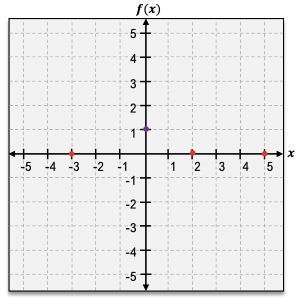
Hey, everyone. We now know how to find a bunch of different individual elements of the graph of a polynomial function, like the end behavior, whether a graph is rising or falling on either end, the x-intercept, where a graph is either crossing or touching our x-axis, our y-intercept, where our graph crosses our y-axis, and how many turning points our graph might have where it changes direction from increasing to decreasing or vice versa. Now, even with all of this great information, we still are missing something. We're not quite sure what's happening in between all of these points. So how do we fill in that missing information in order to give us the complete graph of a polynomial function? Well, here, I'm going to show you how we're going to do that by simply finding and plotting points in these areas that we are not quite sure what's happening yet. So let's go ahead and get started. So because we do have all of these points that we know, we're simply going to break our graph down into intervals of unknown behavior, so these places that I don't know what's happening, and simply find and plot a point in each of these intervals. So, let's take a look at our graph down here. Now, I'm going to go in this graph from left to right, looking at each of my known points and going in between there to create intervals. So looking at my graph starting on this left side going into the right, I'm not really sure what's happening here until I get to this known point of negative 2. So all the way from negative infinity until I get to this point negative 2, I'm not quite sure what's happening. I don't know how steep this end behavior is going to be even if I already know it's going down. So that represents my first interval of unknown information from negative infinity until negative 2. Let's keep going. So from negative 2, where is my next known point? Well, my next known point is going to be my y-intercept at x equals 0. So from negative 2 until I reach that point at 0, which will actually always be a known point of information, I don't know what's happening. I don't know if this is going to be a lower turning point, or it's going to go much steeper. So that represents my next interval. Now from 0, where’s my next known point? Well, it's right here at x equals 3. So from 0 to 3, again, I'm not quite sure what's happening here, so this represents my next interval of unknown behavior. And then finally, from 3 and beyond, again, I'm not quite sure how steep or not so steep this end behavior is going to be, so from 3 to infinity represents my last interval. So these 4 intervals represent all of the places that I don't know the behavior of my graph. I'm not quite sure how steep it's going to be, whether it's going really high or really low. So in each of these intervals, we want to find 1 x value for which we calculate f(x) in order to give us some ordered pair that we can plot on our graph. So inside of my first interval, negative infinity to negative 2, I want to choose a point that I can calculate f(x) for and then plot on my graph. So there is some strategy to picking this point because I don't want to pick something like negative 100 because I'm not going to be able to plot that on my graph, and it's not really going to help me out here. So I want to choose something that is actually going to help me on my graph. So because I have this point negative 2, I might want to know what's happening at negative 3. So I'm going to choose x equals negative 3, and then I would simply calculate f of negative 3, giving me an ordered pair to plot on my graph, giving me some more information in that interval. So moving on to our next interval from negative 2 to 0, in this interval, it might be a little more obvious, some number that we should choose for x. I'm just going to go directly in between at x equals negative 1, and then I would want to compute f of negative 1 in order to give me an ordered pair to plot on my graph. Then into my next interval from 0 to 3 remember, you can choose anything in this interval as long as you're going to be able to graph it. So I'm just going to choose at x equals 2, and then I would simply calculate f of 2 and plot that point on my graph. Then my final interval from 3 to infinity, remember we don't want to choose anything crazy that's not actually going to help us here, so I'm simply going to choose x equals 4, and then I would want to calculate f of 4, giving me my final point of unknown behavior. Okay, now that we have all of these points and we've plotted them on our graph, this is where we would actually want to connect all of these points to give us a clear picture of what's happening here. So with all of that information, I now am left with the complete graph of a polynomial function. Now if you want to plot some more points here, that's totally fine. You can always choose some more values for x to find your f(x) in order to give you an even more complete picture of the graph of your polynomial function. But now that we know everything that we need to graph any polynomial function let's go ahead and get to graphing.

Based on the known points plotted on the graph, determine what intervals the graph should be broken into.  

Plotted points are: $\left(-3,0\right),$$\left(0,1\right),\left(2,0\right),$ & $\left(5,0\right)$

• A. $-\infty\rightarrow-3,-3\rightarrow0,0\rightarrow5,5\rightarrow\infty$
• B. $-\infty\rightarrow-3,-3\rightarrow0,0\rightarrow2,2\rightarrow5,5\rightarrow\infty$
• C. $-\infty\rightarrow-3,-3\rightarrow0,0\rightarrow2,2\rightarrow\infty$
• D. $-\infty\rightarrow0,0\rightarrow2,2\rightarrow5,5\rightarrow\infty$

Graphing Polynomial Functions

Hey, everyone. You now know absolutely everything that you need in order to fully graph a polynomial function. So here, we're going to put all of that together in order to graph a polynomial function from scratch. Now it might feel like a lot and that's okay. I'm going to walk you through it step by step. And if you follow these steps, you'll be able to graph any polynomial function correctly every single time. So let's not waste any time here and get straight into graphing.

The polynomial function that I have here is 2xx3-6x2+6x-2. Now let's start at step 1 and find the end behavior of our polynomial function by looking at our leading coefficient anxn, which in this case is 2x3. So first looking at our leading coefficient an, this is a positive 2. And because this is positive, that tells me that my graph is going to rise on that right side which I can go ahead and sketch here. Then looking at the degree of my polynomial it is 3, which is an odd number, which tells me that the behavior on the end is going to be the opposite. So sketching that on my graph if my right side was rising, the opposite on the left it is going to fall.

Now let's go ahead and move on to step number 2 and find our x intercepts and their behavior. So here we want to go ahead and solve f(x)=0. Now you might have to factor this on your own sometimes, but we already have this pre-factored here so let's go ahead and solve for x. So I'm going to take this factor, x minus 1, and simply set it equal to 0. Now if I add 1 to both sides, it will cancel, leaving me with x equals 1, and that is my single x intercept, x equals 1. Now what is the multiplicity of this x intercept? Well, remember, it's just the number of times that our factor occurs. So here that is 3, which is an odd number. So that tells me that it is going to cross the x-axis at that point. So plotting that on my graph at x equals 1, I know that it's going to fully cross the axis at that point.

Let's move on to step number 3 and find our y intercept. So our y intercept, we're going to go ahead and compute f(0) by plugging 0 into our original function right here. This leaves me with 2×-13, which is really just 2×-1, which is simply negative 2. So this is my y intercept that I can go ahead and plot on my graph. So my y intercept is at negative 2.

Okay. So we've already plotted a bunch of stuff. We have a bunch of known elements. Let's go ahead and move on to step number 4, which is going to be to determine our intervals where we're not quite sure what's happening yet and then plot a point in each of them. So let's determine our intervals by going through our graph from left to right. So looking at that left side and going until I reach my first known point. My first known point is actually my y intercept. So from negative infinity to 0 is going to represent my first interval of unknown behavior. Then going to my next known point here from 0 to 1, which it's really close together, but that's my next interval, 0 to 1. And then, finally, going from 1 and beyond because I don't have any other known points there, from 1 to infinity is that final interval here. So now let's find a point in each of these intervals in order to get a better picture of what's going on in our graph. So in this interval, negative infinity to 0, remember, I want to choose something that's on my graph. So here I'm going to go ahead and choose x is equal to negative one to get that point. Then from 0 to 1, this is a rather small interval, so it is okay to choose a fraction here. I'm gonna go ahead and choose 1/2 in that interval. Then from 1 to infinity, remember again, I don't want to choose anything too crazy. That's not actually going to help me. So I'm simply going to choose the point x equals 3. Now you can go ahead and pause here and plug each of these into your function in order to get f(x) and then come back and check that you've got the same answer as me. So here, for x equals negative 1, if I plug negative 1 in, I'm going to end up with negative 16. So the first point that I can plot here is negative 1, negative 16. Then 1/2 if I plug that into my function, I will end up getting a negative 1/4, which I can also go ahead and plot on my graph. Now I know that that doesn't look like it helps a ton here but it was an unknown interval. And then lastly, I have this x equals 3, which if I plug in, I end up getting positive 16, which is the last point that I'm going to plot here, at 3, positive 16.

Okay, now we have a ton of information about our graph, and it looks like we can go ahead and move on to step number 6 and simply connect all of our points with a smooth and continuous curve because it's a polynomial function. So starting with the point that I have up here, I'm gonna go ahead and connect with a smooth curve all of my points. Now you'll notice that I didn't go through those original end behavior lines and that's totally okay. I still am matching the end behavior. I just found out some more information so I can sketch it more accurately. So we're completely done. We have finally fully graphed our polynomial function.

Let's perform one final check here using our turning points. So with our turning points, remember, the maximum number we can have is our degree minus 1. Here my degree is 3, so 3 minus 1 gives me a maximum number of turning points of 2. Now looking at my graph, does this have more than 2 turning points? No. It doesn't even have one turning point so my last check is good and I am completely done. Now you have fully graphed your polynomial function let's get some more practice.

Example 1

Hey everyone. Now that we know how to fully graph a polynomial function, let's work through this example together and graph this polynomial function, and then determine both the domain and range. The function I have here is f(x) = 3x^3 + 12x^2 + 12x. So jumping into step 1 determining our end behavior, we want to go ahead and look at our leading term here which is 3x^3. Now the very first thing I want to look at is my leading coefficient which in this case is 3, and it is positive. So that tells me that the right side of my graph is going to rise. Now because my degree here is 3, this is an odd number that tells me that the ends are going to have the opposite behavior. So going ahead and sketching that on my graph here, I know my right side is going to rise, and then my left side is going to do the opposite because the ends have the opposite behavior. Remember that this doesn't need to be precise yet, we're just sketching what's eventually going to happen on our graph. So we're done with step 1. Let's move on to step 2 and determine our x intercepts and their behavior. Now for this one we need to do a little bit more work and do some calculations, so let's go ahead and set up our equation f(x) = 0 so that we can solve that. Now I'm gonna take my function here, which is 3x^3 + 12x^2 + 12x and set it equal to 0. Now let's come down here and work this problem out. So looking at this function or this equation that I have here, I see that I can go ahead and factor out a greatest common factor out of each of these terms. Now they all have the common factor of 3x that I can go ahead and pull out. So taking out that factor, I'm left with x^2 + 4x + 4 = 0. Now here I don't have to worry about this 3x anymore, but I can further factor this. And you may recognize that this is a perfect square trinomial. So I can actually factor this into (x + 2)^2 = 0. So now this is fully factored, and I can go ahead and take each factor and set them equal to 0. So I have 3x = 0 and then x + 2 = 0. Now solving for x in each of these, this 3 isn't going to do anything. I'm simply left with x = 0. And then over here, I can subtract 2 from both sides, canceling that out, leaving me with x = -2. So these are my 2 x intercepts, x = 0 and x = -2. Now we need to determine the behavior of the graph at each of these points, so we wanna look at the multiplicity. Now looking at my x = 0, I see that it comes from the factor 3x, which only occurs once. So this has a multiplicity of 1. Now 1 is an odd number, so that tells me that my graph is fully going to cross the x-axis at that point. Now looking at my other factor x = -2, I see that this comes from the factor x + 2 which is squared. So this happens twice. It has a multiplicity of 2. Now because that multiplicity is even, that tells me that my graph is simply going to touch the x-axis and bounce right back off at that point. So we have our x intercepts and their behavior. Let's go ahead and put them on our graph. So looking at x = 0, I know it's going to cross the x-axis at that point, and then x = -2. It is only going to touch and bounce off, which might be shaped something like this. Remember that we're just sketching this right now. We'll connect it all with more information later. So we have our x intercepts. Let's move on to look at our y intercept, which we can find by calculating f(0), plugging 0 into our function. Now we can go ahead and use our factored version here. We have this 3x \times (x + 2)^2, or you can always go back to your original function and plug 0 in there. I'm gonna use the factored version here because I think it's gonna be a little bit easier. So plugging 0 in, I get 3 \times 0 \times (0 + 2)^2. And now all of this is getting multiplied by a 0, so that tells me that I'm simply going to be left with 0 here. So my y intercept is just 0, which I don't need to plot on my graph because I already have it at that origin point there from my x intercept. Now that we have those done, let's move on to determine our intervals. So let's take a look at our graph. Now we wanna go in our graph from left to right looking for points that we know and identifying those intervals of unknown behavior. So from negative infinity until I reach my first known point, I first know something at x = -2. So my very first interval is from negative infinity until I reach -2. Then going from -2 until I reach my next known point, it is at x = 0. So my next interval is simply -2 to 0. And then finally from 0, there is no other known point on my graph, so my last interval is from 0 all the way to infinity. Now that I have my intervals of unknown behavior, I'm gonna go ahead and identify a value for x in each of those intervals that I can calculate a point for. So my first interval from negative infinity to -2, I wanna choose a point that I will be able to plot my graph, which here I'm just gonna go ahead and choose -3. Then from -2 to 0, I'm just gonna go ahead and choose a point right in the middle of that interval at -1. Then finally from 0 to infinity, I'm just gonna see how quickly it increases from there, and I'm gonna go ahead and choose x = 1. Okay. Now that we're here, we wanna take each of these x values and plug them into our function to calculate f(x) to get that ordered pair. So let's come down here and plug all of these into our function. I'm first going to calculate f(-3) by plugging -3 in for x to my function. Now again, you can use your factored form or you can use your original equation. I'm again gonna use the factored form because I think it'll make it a little bit easier. So here I have 3 \times -3 \times (-3 + 2)^2 equals this 3 \times -3. I can go ahead and combine that. That's gonna give me -9. And then I have -3 + 2, which is going to give me -1, and that is squared. Now -9 times -1 squared. -1 squared is just 1, so this is just -9. And that's my first ordered pair, -3, -9. Now for my next ordered pair, I'm gonna calculate f(-1) by plugging -1 into my function. So 3 \times -1 \times (-1 + 2)^2. And simplifying that, 3 \times -1 is going to give me -3. And then -1 + 2 gives me +1, and that is squared. One squared is just a one, so this is just -3 times 1, which is -3. And here's my second ordered pair, -1 -3. Now lastly, I need to go ahead and calculate f(1). So plugging 1 into my function, I get 3 \times 1 \times (1 + 2)^2. And simplifying that, 3 \times 1 is just 3. 1 +2 is also 3, but that 3 is squared. So this becomes 3 \times 9 because 3 squared is 9. 3 \times 9 is 27. So we have our final ordered pair here, 1, 27. So we're done calculating those points. Finally, let's go ahead and put them up on our graph here. So my first point is -3, -9, which I can go ahead and plot -3, and then -9 is right around here. And then my second point I have is -1, -3, which plotting that -1 and -3. So right about in the middle there. And then finally 1, 27. So we see that this increases really quickly on this side, 1 all the way up to 27. Now filling in those unknown behavior I can now finally connect everything with a smooth and continuous curve like I know all polynomial functions have. So let's go ahead and connect everything using what we already know. So we know that our end behavior is gonna go down to negative infinity on this side, and then we're gonna go through this point and cross and all the way up. Now remember, it's okay if your curve isn't perfect. It can be really hard to draw these in a continuous line. I'm gonna go ahead and remove all of that extra stuff on my graph so I'm just left with my final graph. Remember the other step is just to help us later on so that we can really easily sketch this at the end. So here's my polynomial function. We still have one last thing to check here and that is our turning points, which we want to make sure does not exceed our maximum number. Now for our turning points, we wanna take our degree, which is 3 here, subtract 1, which gives us 2, and check that we don't have more than 2 turning points here. So I see that I have a turning point right at -2 and then somewhere around here is another turning point. I don't have any more here, so it looks like I'm good. I have not exceeded my maximum number of turning points. Now we have finished everything with our graph, but we're gonna take a look at our graph and determine 2 more things, our domain and our range. Now remember the domain, we actually don't have to determine anything because the domain of all polynomial functions is the same. It is negative infinity to infinity, or all real numbers. Now for our range, we do want to take a look at our graph here because it can vary based on our function, but we know that it continues on to negative infinity down here on the bottom. And then on the top, we see that this also carries on to positive infinity. So our range is actually going to be the same as our domain here and go from negative infinity to positive infinity. Now that's not always going to happen with every single polynomial function, it just happens to happen with this function. So we finally have graphed our full polynomial function and identified our domain and our range. Let's get some more practice.

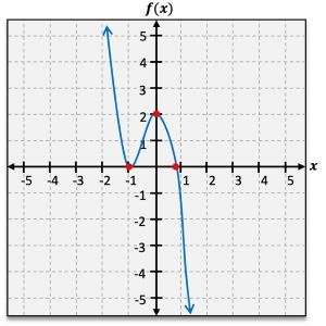
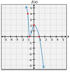
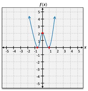
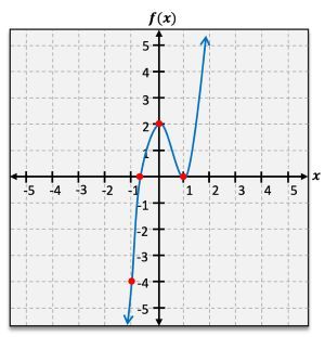
Graph the polynomial function. Determine the domain and range. $f\left(x\right)=\left(3x+2\right)\left(x-1\right)^2$

• A.
• B.
• C.
• D.

Here’s what students ask on this topic:

How do you determine the end behavior of a polynomial function?

To determine the end behavior of a polynomial function, examine the leading term, which is the term with the highest degree. The end behavior is influenced by the leading coefficient and the degree of the polynomial. If the leading coefficient is positive and the degree is even, the graph rises on both ends. If the leading coefficient is positive and the degree is odd, the graph falls on the left and rises on the right. Conversely, if the leading coefficient is negative and the degree is even, the graph falls on both ends. If the leading coefficient is negative and the degree is odd, the graph rises on the left and falls on the right.

What is the significance of the multiplicity of x-intercepts in graphing polynomial functions?

The multiplicity of an x-intercept in a polynomial function indicates how the graph behaves at that intercept. If the multiplicity is odd, the graph crosses the x-axis at that intercept. If the multiplicity is even, the graph touches the x-axis and turns around at that intercept. For example, if a polynomial has a factor of (x - 2)³, the graph will cross the x-axis at x = 2 because the multiplicity is 3 (odd). If the factor is (x - 2)², the graph will touch and turn around at x = 2 because the multiplicity is 2 (even).

How do you find the turning points of a polynomial function?

The turning points of a polynomial function are points where the graph changes direction from increasing to decreasing or vice versa. The maximum number of turning points is one less than the degree of the polynomial. For example, a polynomial of degree 4 can have up to 3 turning points. To find the turning points, you can take the derivative of the polynomial and set it equal to zero to find the critical points. Then, determine whether each critical point is a maximum, minimum, or neither by using the second derivative test or analyzing the sign changes of the first derivative.

How do you graph a polynomial function step by step?

To graph a polynomial function step by step, follow these steps: 1) Determine the end behavior by examining the leading term. 2) Find the x-intercepts by solving the equation f(x) = 0 and note their multiplicities. 3) Find the y-intercept by evaluating f(0). 4) Break the graph into intervals of unknown behavior between the intercepts. 5) Choose points within these intervals, calculate their f(x) values, and plot them. 6) Connect all points smoothly, ensuring the graph reflects the polynomial's characteristics, including turning points. 7) Verify the graph by checking the maximum number of turning points, which should not exceed the degree minus one.

What are the key elements to consider when graphing a polynomial function?

When graphing a polynomial function, consider the following key elements: 1) End behavior, determined by the leading term's coefficient and degree. 2) X-intercepts and their multiplicities, indicating where the graph crosses or touches the x-axis. 3) Y-intercept, found by evaluating f(0). 4) Turning points, which are the points where the graph changes direction. 5) Intervals of unknown behavior, where additional points should be plotted to understand the graph's shape. 6) Smooth and continuous connection of all points, ensuring the graph accurately reflects the polynomial's behavior.