Introduction to Matrices: Study with Video Lessons, Practice Problems & Examples

Understanding matrices is essential for solving systems of equations. A matrix organizes coefficients into a grid format, with row operations like swapping, multiplying, and adding rows to manipulate the data. The goal is to achieve row echelon form, characterized by ones along the diagonal and zeros below, or reduced row echelon form, which also requires zeros above the diagonal. This process, known as Gaussian elimination, simplifies solving equations, allowing for straightforward back substitution to find variable values.

Introduction to Matrices

Everyone, welcome back. So, we've spent a lot of time talking about systems of equations in the last few videos. We're going to shift gears a little bit. We're going to start talking about a new idea called a matrix, or the plural version is matrices. Now matrices can seem kind of scary at first because you'll see these big blobs of brackets with numbers inside them and all that stuff. But I'm actually going to break it down for you, and I'm going to show you that a matrix is really just a way to organize information or numbers into a grid-like pattern with rows and columns. Alright? So let's go ahead and get to it. I'm going to break it down for you. Alright? So we've got this matrix here, and the way we sort of define a matrix or we label the these parts of a matrix is by rows and columns. There are 2 rows in this matrix. We have 1 and 2. Those go horizontally, and we also have 3 columns in this matrix. Right? So 3 columns. So this is just 1 2 3. Alright? Now, so you might see this matrix referred to as a 2 by 3 matrix, 2 rows, 3 columns. Alright? Now, really, all this matrix is is just a way to sort of arrange numbers, and you'll actually see that the numbers are the exact same that they are in the system of equations over here. In this system of equations, we had 2 equations, and those things just became our 2 rows in our matrix. We also have three numbers in the columns, 2 for the coefficients and then one for the constants over here. Those three numbers really just became our 3 columns over here. So really, it's just a way to represent this information that's in the system just in a different way. Alright? And when you do this, when you have a system of equations represented as a matrix, it's called an augmented matrix. That's just a sort of a fancy word that you'll see in your textbooks and here in your classes. That's all that really means. Alright? So all we're really doing here is we're just sort of copying over the coefficients into this matrix, and we're sort of leaving out the variables. So we have negative 72. That becomes negative 72. Then we have this negative 3 and onetwo. That's negative 3 and onetwo. And then this negative 4 and 13 just becomes negative 4 and 13. So we're just copying over all the numbers, but we're just leaving out the coefficients. Because in a matrix, it's understood that these columns mean x and y coefficients. Now what you'll also see is you'll see this little black bar that's inside of these matrices, and this just means an equal sign. That's kind of what that means. So you'll see here that the really, a matrix is just a more compact way to represent all of the information that was in the system of equations. Alright? That's really all there is to it. Later on, we'll learn different ways to manipulate matrices and even do some operations with them. But for now, all we need to do is basically just turn a system into a matrix. Let's go ahead and take a look at an example problem here. So we're going to take this 2x plus 3y. So we're going to take this system of equations and represent this as a matrix. So we've got 2x plus negative 3y equals or, like, plus z equals negative 4. And then we got 6x plus 3y equals 13, and then y minus z equals 8. Alright? So it's really important that you actually lay out when you have a system of equations so that you have the coefficients and the variables that are on top of each other, x's with x's, y's with y's, and z's with z's. And so that's one of the things you may have to do before turning something into a matrix. Alright? But remember, really, all we're going to do is we're just sort of going to extract out the coefficients. So I'm going to have 3 columns here because I have 3 variables. Actually, I'm going to have 4 columns because I have 3 variables plus one constant on either side. So this is going to be like, the constants over here. Alright? So if you look at this first equation, what happens is I have a 2 in the x, negative 3 in the y, and then 1 in the z. So this is just going to be 2, negative 3, and then 1. The constant that goes on the other side is going to be negative 4. Alright? So that's for that first equation. Let's take a look at the second one. The second one has 6 in the x, 3 in the y, so 6x3y. But what about the z components? Here, we had one z over here. What happens if we just see nothing? Well, really, if you ever just see a blank space, it actually just means that there is, like, 0 z there. There's, like, a 0 there. So you don't just leave the matrix empty. You actually will just put a 0 there. Alright? So this will be 13. And then finally, what we're going to have is y minus z is 8. So here now what happens is that we have no x components. There's no x coefficient, so we just label that as 0. Then we have here is 1, and then minus z means negative 1. And over here, we have 8. So this is how you take this system of equations here and represent this as a matrix. So this would be the augmented matrix for this system of equations. Alright? That's it for this one, folks. Thanks for watching. I'll see you in the next one.

Write the equations in standard form, then represent the system using an augmented matrix.

$3x+5y-9=0$

$8x=-4y+3$

• A.
• B.
• C.
• D.

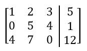
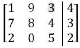
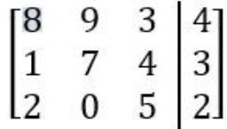
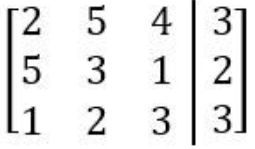
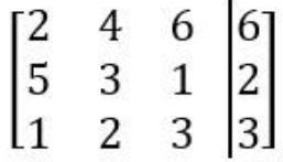
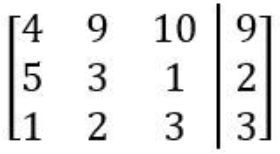
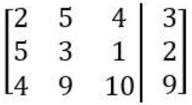
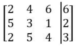
Write the system of equations represented by the augmented matrix shown.



• A. $x+2y+3z=5;5y+4z=1;4x+7y=12$
• B. $x+2y+3x=5;5x+4y=1;4x+7y=12$
• C. $x+2y+3x=5;5y+4z=1;4y+7z=12$
• D. $x+2y+3x=-5;5y+4z=-1;4x+7y=-12$

Performing Row Operations on Matrices

Welcome back, everyone. So back when we studied systems of equations, we saw lots of different ways to manipulate those equations. For example, we saw that we could swap the positions of 2 equations. We could also multiply equations by some number, like when we did the elimination method. We can also add equations together once we had those coefficients to be equal and opposite. Well, remember that a matrix is really just a representation of a system of equations. It's just two ways of writing the same information. So just as we did operations to these types of equations, we can also do operations on the rows of a matrix because remember, an equation is really just a row on a matrix. So we call these things row operations. What I'm gonna show you in this video is that there's really just three of them that you need to know, and I'm gonna break it down for you, showing you a bunch of examples. Alright? And there's also some new notation we'll learn as well. Let's get started with the first one, which is swapping 2 rows. This is by far the easiest operation, and it sounds exactly like what it sounds like. Right? We're just gonna be swapping the position of 2 rows just like we swap the position of 2 equations. So, here, all that happens is that we had -1, 2, and 9 on the top row, and now it just goes to the bottom. So this is -1, 2, and 9. And then the 2, 6, and 12 that was on the bottom, now it just goes to the top, 2, 6, and 12. Now you'll see some notation for this written in your textbooks with some little r's and big R's. Really, all this stuff says is little r means the old row, and big R means the new row once you're done doing that operation. And the subscripts just tell you which number or which row they're talking about. So, for example, this is little r one over here, and that little r one becomes big R two and vice versa. This little r two becomes big R one. So that's really all that's going on there. It's just showing you old versus new and the number of the row that it is. Alright? So that's the first one. Let's take a look at the second operation, which is multiplying one row by any non-zero number. Alright? So when we dealt with the system of equations in the elimination method, we could multiply an equation by some number. So, for example, we multiply this by 2. And what happens is we change all the coefficients. This would be -2x and this would be 4y, and this would be 18. Well, we can do the exact same thing to the rows or the numbers in the rows of a matrix. So really all this is we're going to take this little r two over here, and the notation for this is we're going to take little r two multiplied by 2, and that becomes now big R two. We're just gonna rewrite this new row. Alright? So what happens is we're gonna take all these numbers, multiply them by 2. This may ends up being -2, 4, and 18. Notice how all these numbers are the same because remember, this matrix is just representing the system of equations. Alright? Alright. So these numbers here are all the same. Alright. So, let's move on to now the last one, which is just adding some multiple of one row to another. Alright. So when we did this for systems of equations and we finally got their coefficients to be equal and opposite, we could add the equation straight down and cancel out or get rid of 1 of the variables. What we were left with is we were left with something like 10y equals 30. So now what we can do here is, with a matrix, we can do the same exact thing. Now when we did the first system, we always just delete or not even rewrite that first equation because we're only just worried about that one equation here. With the matrix, you can't just sort of delete a row, so you just rewrite it. Right? So the 2, 6, and 12, you just rewrite the 2, 6, and 12. Alright? But now what you're gonna do here is you're gonna take this little r 2. You're gonna take this little r 2, and I'm just gonna add it to all the other numbers in little r one, and I'm just gonna add these things straight down. And that now becomes my big R 2. So, this should become 0, 10, and 30, and you're gonna get exactly the same sort of numbers that you get on left and right. It's just another way to represent this system of equations. Now, unfortunately, this step here of adding, some kind of a non-zero multiple of one row to another is actually, unfortunately, the most common step, so it's good to get some good practice with this. I also want to mention one other thing here. The last two steps that we talked about are operations, the multiplying and adding. They only affect one row. It's the row that they're you're currently doing an operation on. The only time you're actually doing 2 rows or you're affecting 2 rows is when you're swapping them. So what you'll see here is that we rewrote, for example, the 2, 6, and 12. We changed we never it never changed the entire time. And that's because the only row that was changing was row 2. Alright? So, anyway, those are the 3 operations. Let's go ahead and get some more practice here using, this this, this sort of more a little bit more complicated matrix. So here we've got 2, -6, 4, 10. We've got this big matrix over here. Let's take a look at the first one. The first one says we're gonna take row 2, and we're gonna swap it with row 3. So remember, this is just the notation for swapping. So all we're gonna do here is this is gonna be my r 2. This is gonna be, sorry. This is gonna be that's gonna be r 2, and now it's just gonna trade places with the 3rd row. Alright? So just gonna rewrite this matrix over here. Remember, this the first row is gonna remain completely unaffected. So this is 2, -6, 4, 10. Just rewrite it. Now what happens is the 3 eights, -7, and 0, will actually go to the bottom. 3, 8, -7, and 0, and now what happens is the this row over here will go to the top. So this is gonna be -1, 5, 9, and 3.

Perform the indicated Row Operation.

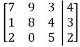
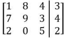
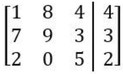
SWAP $R_1\leftrightarrow R_2$

• A.
• B.
• C.
• D.

Perform the indicated Row Operation.

ADD $R_1+2\cdot R_3\rightarrow R_1$

• A.
• B.
• C.
• D.

Solving Systems of Equations - Matrices (Row-Echelon Form)

Welcome back, everyone. In the last few videos, we've learned the row operations that you can perform on the rows of a matrix, like swapping, multiplying, and adding. And I mentioned that we would eventually use those to solve a system of equations. Well, that's exactly what we're going to do in this video. We're going to solve the system of equations by getting a matrix in a very particular form that we'll discuss in just a second. The whole idea is that I'm going to take a system of equations, turn it into a matrix, and then use row operations to get a very particular pattern of numbers of ones and zeros. And then, once I get that, I can turn it back into a system of equations and then solve it that way. Let's go ahead and take a look here. The first time you see this, it might be kind of intimidating, but I'm going to break it down for you, and we'll work out this example step by step. Let's get started here.

The whole idea is that we're going to use these row operations to get a matrix with ones along the diagonal. So notice how I have this sort of diagonal here from top left to bottom right, and then I have zeros underneath the diagonal. That's really what you're trying to get, ones along the diagonal and zeros underneath. Now, remember, these coefficients represent the coefficients of a variable in a system of equations. So the reason you want to get to this in this form, which is, by the way, called row echelon form, is because once you turn it back into a system of equations, what happens is that you're just going to get equations that you can substitute and then solve for x and y using that method. It really just turns into a regular system of equations problem, which we've seen how to solve before. I want to mention here that these numbers can actually be anything. There are no restrictions on them so that they don't have to be ones and zeros or anything like that.

What I'm going to do is I'm actually going to break this example down. We're going to work this out together. I'll show you step by step how we get to this row echelon form. Alright? Let's take a look. So, I've got my system of equations over here, \( -x + 2y = 4 \), \( x + 7y = 14 \). In fact, it's actually the same system of equations I had over here. So I'm really just going to start by turning it into a matrix and copying this over. So this is \(-1, 2, 4; 1, 7, 14\). I've got my augmented matrix over here. The goal is I want to get ones along the diagonal and zeros everywhere else. Here, I've got a negative one and seven along the diagonal, so I need to get a one in this position. And that actually brings me to the first tip here. I'm going to give you some tips for solving these problems, and the first one is just to go row by row and work your way top to bottom.

To get a one in this position, let's consider each row operation. Can I swap two numbers over here to get a one in this position? Well, actually, you can because notice how this is a negative one and a positive one. So if you swap these two rows, then you'll get a one there. So that's the first thing you can do. You won't always have to do that; it's just, in this case, we can swap because we've seen that there's a one in this position. So we're going to swap row 1, and that will just become my new row 2. So, really, all that happens is that these rows just switch places. So this is 1, 7, and 14 now; \((-1, 2, and 4)\). And now, all of a sudden, we can see that we have a 1 in this position. That's one of our numbers. Alright? So now we just have to focus on these two numbers. This has to become a 0, and this has to become a 1. We're going to use row operations to do it.

You might be thinking that we'll just stick with trying to get the ones along the diagonals. But actually, what I'm going to show you here is that trying to get this one isn't going to be the right move. Because what happens is if you try to get this position here to be a 1 by multiplying this equation by, let's say, \(\frac{1}{2}\), then this will become a 1 but this will become \(-\frac{1}{2}\). And you're going to end up with a weird negative fraction here. Then later on, to try to get rid of it, you're going to have to mess up the one that you've already gotten. Instead, what happens is that brings me out to my second tip. Whenever you get a one along the diagonal, you would want to get everything underneath it to be 0 before you move on and try to get to the next one. What do I mean by this? Now that we've gotten this first one, I'm going to focus on getting this number to be 0 before I focus on getting this to be a 1. And we're going to see why that works in just a second.

So how do I get this one to be a 0? Well, can we swap? Well, swapping is going to be pretty silly because we're just going to undo all the progress we've already done here. So that's not going to work. So what about multiplying? Well, the only way we could get a 0 out of this is if I multiply the entire row by 0, but I can't do that because I have to multiply rows by non-zero numbers. So multiplying isn't going to work either. The only way to get a 0 in these types of problems is you're going to have to add. By the way, this is always going to happen. So to get zeros, you're going to have to always add something. Alright? So here, what we're going to do is we're going to take row 2. We're going to have to add it to something to get a 0 in this position. What do I have to add to this to get it to cancel out to 0? I just have to add 1. And that's exactly what I have in the first row. So remember, I can multiply or I can add a multiple of a row. But in this case, all I have to do is just add row 2 and row 1 together with no multiple, or otherwise, just 1 times row 1. And that's going to be my new row 2.

So now what happens here is, remember, that row operation will only affect row 2, so row 1 will remain completely the same. \(1, 7, and 14\) doesn't change. Now what happens here is I'm going to add these coefficients down. \(1\) and \(-1\) becomes \(0\), \(7\) and \(2\) becomes \(9\), and then \(14\) and \(4\) becomes \(18\). Now if you see what happens here, I've got a \(1\) in this position, and I've got a \(1\) underneath it. So that's good. I've gotten 2 of my numbers. I really only have one thing to do left, and that's I have to turn this thing into a one. Alright? So how does that work?

Well, whenever you're trying to turn numbers into ones, you're not going to add. You're going to actually multiply. Because now what I can do in this problem is I can multiply this whole entire equation here by whatever I need to get this to be a 1. And I really just have to multiply this entire equation here by \(\frac{1}{9}\). So what I'm going to do is I'm going to multiply, \(\frac{1}{9} \times r_2\). Now the reason this is helpful is because notice how multiplying this equation won't actually affect the \(0\) because \(\frac{1}{9} \times 0\) is still \(0\). So this is why multiplying to get ones is going to be easier. So here what happens is this is going to be \(1, 7, and 14\), and this is going to be \(0\). So I've got \(0\) over here. This becomes a \(1\). And then if I multiply \(18\) by \(\frac{1}{9}\), that actu

Example 1

Hey, everyone. Welcome back. So in this problem, we're going to take this system of equations that we have given to us right here, and we're going to solve it using row operations. And the key thing here is, remember, when we use row operations, we're trying to get a matrix in row echelon form. And remember what that looks like. Row echelon form means that we have a matrix with all ones in the diagonal, and we have all zeros under the diagonal. And remember that these numbers over here that are sort of above and to the right of the diagonal, they can be anything. There's no restriction on them.

So we're going to have to take this system of equations and turn it into a matrix first so that we can start doing that. Let's get started here. The first thing is we're going to convert this into a matrix. And, really, we've done this before. We just have to pull out the coefficients. So this is going to be 1, 3, 4, and 2. This will be 2, 5, 7, 9, and then 4, 8, 10, and then this is going to be 14. Alright? So if you look here, I've already actually gotten one of the numbers that I need. I've gotten one of the ones in the diagonal, so it's a little bit of a head start, which is good.

Now what we have to do is we have to focus on these numbers. I want these to be ones, and then I want these numbers, the 2, 4, and the eights. I want those things to become zeros. And how do I do that? I'm going to have to use all the row operations that we've learned in order to get that system of equations or that matrix in row echelon form. Let's go ahead and get started here.

Now you might think that you should focus on any number. Like, for example, you could focus on this 5 or the 10. But remember that second tip that we discussed in the video. Obviously, you always want to work down sort of from top to bottom in your equations, but you also every time you get a one, you want to make sure that you get all these numbers to be 0 underneath the diagonal, or underneath that one before you start focusing on the next one. What happens is if you try to make this one, then you're going to affect this cell over here, this number. And then later on, you're going to have to sort of get this to be 0, and then you're going to have to sort of mess up the one that you've already gotten. So it's always better to get this thing to be 0 or these numbers to be 0. Let's go ahead and do that.

Alright? So how do I get this number to be 0? Well, I can't swap because nothing was going to get me a 0 in that place, and I can't multiply this thing. I have to multiply this whole entire equation by 0. So The only thing I have to do is the only thing I can do is I can add. So I'm going to have to add something to row 2 in order to make it 0. So how do I do that? Well, the only number that's going to make this 0 is if I add it to negative 2. So I'm going to have to add so row 2 to some multiple of some equation in order to get a new row 2, and that's going to give me a 0.

Now one of the reasons it's nice to get ones in these, equations is because then you could just multiply them by a number, to get something to cancel out with this number over here. So for example. So I've got this 2. I need it to cancel out by becoming by adding it to negative 2. So what I can do is I can take this whole entire row, and I can multiply it by negative 2. So I'm going to do negative 2 times row 1 and then add it to row 2, and that's going to become my new row 2. Let's work it out real quickly and just see how this works.

So this row 2 that I have is just equal to 2, 5, 7, and 9. Right? That's what that row is. What about negative two times row 1? Take all the numbers that you see over here and multiply them by negative 2. What do you get? I'm going to get negative 2, and I'm going to get negative 6, and I'll get negative 8, and then negative 4. Alright. So you multiply all those numbers. Now what happens is when you add these 2 rows, what you'll see is that the 2 and negative 2 will cancel, leaving you with just 0. The negative 6 and 5 becomes negative 1. Negative 8 and 7 becomes negative 1, and the negative 4 and 9 becomes 5. So this over here is actually what your new row 2 is.

Alright? So now let's go ahead and rewrite this matrix. And remember, the only thing that gets affected here is just this row 2. So let's rewrite this. So this is going to be it's going to be 1 3 4 2. And then remember, the 3rd row is going to be unaffected, so 4, 8, 10, and 14. But now the 2nd row gets rewritten. So 0, negative 1, negative 1, 5. Alright? Now if you look here, we've actually made some progress. I've got a one here, and then I've got a 0 over here. So it's making some progress. And if you actually look, this number is really close to being the one really close to being the one that we need along the diagonal, but it's negative. But we'll focus on that later. Remember, what we also want to do is we want to keep on working down the equations and getting all the numbers underneath the ones to be zeros.

So now let's take a look at this third equation. You actually see that we're going to do something very similar. I'm going to have to get this to be 0, so I can't swap it. Otherwise, or I could swap it, but then I'm going to have to deal with the row that I just messed up, and so that's not going to be a good idea. I can't multiply this, so I'm going to have to add it to something. I'm going to have to add something to row 3 in order to get these numbers to cancel. So I'm going to add row 3 to something. Now just like I multiplied the first equation by negative 2 to cancel out the 2 that was here, I can do the exact same thing. I can instead multiply row 1 by negative 4. So then I'll get a negative 4 that cancels out with a positive 4. Alright?

So over here, what I'm going to get is negative 4 times row 1. So let's do this over here. Row 3 was equal to I had 4, 8, 10, and 14. If I take negative 4 multiplied by row 1, what do I get? I get negative 4, and then I'm going to do everything in this. I'm going to take every number here, multiply by negative 4. So it becomes negative 12, this becomes negative 16, and this becomes, negative 8. Alright. So if you add these two things, you're going to get this new row 3, which is going to equal well, the 4 negative 4 will cancel, which is exactly what we would expect. The negative 12 and 8 becomes negative 4. The negative 16 and 10 becomes negative 6, and this becomes positive 6. Alright? So this is what your new row 3 is now.

So again, let's rewrite this matrix, and we're going to see that we've made a little bit more progress. We've got 1, 3, 4, and 2. We've got 0, negative 1, negative 1, and 5. And now we've got 0, negative 4, negative 6, and positive 6. So we basically just rewrite these new matrices once we've calculated that. Alright? Okay. So now we've got 1 and we've got a 0 and a 0. So, again, making some progress. You just take it one step at a time.

So now let's go ahead. And now that we've gotten all these numbers underneath the first one to be 0, now we can start to focus on the next one. So let's look at the second equation over here, and we'll see that this number here has to become 1. So let's go through the steps. Can we swap anything? Well, we don't want to swap because then we're going to mess up the first two rows. Right? So can we multiply something by can we multiply this equation by something to get me 1 in this position?

And we actually can. So we can actually multiply over here. So I'm going to multiply. What do I have to multiply this whole equation by to get a one in this position? Well, I have a negative one, so I could just multiply by negative one. So this is just going to be I'm going to take row 2, and I'm going to multiply negative one times row 2, and that will become my new row 2. Alright? So this is pretty straightforward. Let's just go ahead and do this real quick.

So again, this is going to be 1, 3, 4, 2, 0, negative 4, negative 6, and 6. Those 2 rows get unaffected. But now what happens is if I multiply everything in this row by negative one, then everything just flips signs. So I get 0, 1, 1, and negative 5. So now let's look here. I've got a one here and a one here, and I've got 0 here and 0 here. So I'm very, very close. Alright. So now what do I do? Well, every time I get a one, I want to get all the numbers underneath it to be 0.

So, again, can't swap, can't multiply, but now we can add. Alright. So we're going to add something to this 3rd row. So we're going to add something over here in order to get this negative 4 to cancel out. So I'm going to add row 3 to some multiple of something in order to get that negative 4 to cancel. Alright? So what do I multiply by or, sorry, what do I add, what do I add to this equation? Can I add it to some multiple of row 1? Well, what happens is if I try to, then if I multiply by or if I multiply this row by 1, then I'm going to get negative 4 +3, and that's not going to cancel out to 0. If I try to multiply this thing by 2, then then that's going to be 6, but that's going to be too much. So I can't, I can't do row 1.

Instead, what I can do is I can use the one that I just got above. Just cancel out this negative 4. So what I can do is I can multiply this row 2 by 4, and then this would become my new row 3. Okay? So let's work that out. So row 3 is remember, this is just, 0, negative 4, negative 6, and 6. And now if I do 4 times row 2, what is that matrix, or what is that row? Well, 4 times 0 is still 0. 4 times 1 is 4. 4 times 1 is 4, and then 4 times negative 5 is negative 20. Alright?

So if you add those two things, that should become your new row 3. And what does this become? Well, the zeros don't actually do anything. They still say 0, which is great. And then the 4 and negative 4 will cancel out to 0. That's also good. The 4 negative 6 become negative 2, and then this over here becomes negative 14. Alright? So that's negative 14. Okay.

So now this becomes my new row 3, and I'm just going to rewrite this matrix. So again, these problems are very, very tedious. We'll just go through 1 at a time, sort of just chip away at the numbers, and we'll go ahead and solve it. Alright. So this becomes 1, 3, 4, and 2. Notice how this first equation actually hasn't even changed at all. Now this becomes 0, 1, 1, and negative 5 over here. And now what we got here here is 0, negative 2, and then negative 14.

So now if you look here, I've got 1, 1, and then I've got 0. I've got all the zeros taken care of. And the last thing I can do here is I can just focus on getting this last one. And if you look at it, this is going to be pretty straightforward because all I have to do is just get this negative 2 to become positive 1. How do I do that? I'm not going to add. I could just multiply. Alright? So I could just multiply this whole entire equation. So we're going to multiply again, And what we're going to do here is we're going to multiply this whole entire equation by negative one half. The one half will make it 1, but then we have to multiply by negative to cancel out the negative sign.

So there's going to be negative one half times row 3. That will become my new row 3. And then this will finally be I've got 1, 3, 4, and 2, 0, 1, 1, and negative 5, and then I've got 0, 1, and 7. Alright? Now that we've gotten these numbers, I've got my equation or my matrix in row echelon form. I've got ones along the diagonal, and then I've got zeros under the diagonal. And remember, these over here can be any number. Now what's the last step is now we actually have to convert it back into a system of equations.

All right. So we're basically almost done, homestretch. We just turn this back into a system of equations, and this just becomes x plus 3y plus 4z, and that equals 2. Now in the second equation, we have y plus z equals negative 5. Basically, just pulling the coefficients back into just or these numbers back into coefficients of an equation. And then this final one over here, this last equation, remember, these just are x and y and z coefficients. This just becomes z equals 7.

So how do I figure this out? How do I solve this? Well, you basically just sort of work your way back up the chain and then sort of plug stuff into the equation before it. So I'm going to call this equation 1, equation 2, and equation 3. If you plug the equation 3, the z equals 7 back into equation 2, what do you get? You get y + and then remember z is equal to 7 now, so y + 7 is equal to negative 5. If you go ahead and solve for this, what you're going to see is that y is equal to negative 12.

So that's the that's one of the numbers that you have, or that's one of the sort of the answers to this problem, z equals 7. When you plug it back into equation 2, you get the second number, which is y equals negative 12. And then when you take both of these numbers and plug it back into equation number 1, you'll get your 3rd number. So equation 1 becomes this. So this is going to become, x plus 3. Now we don't plug in y because we know y is equal to negative 12. And we don't plug in z because we know that z is equal to 7, and this is equal to 2. Alright?

So if you solve for this, what you're going to see is that you end up getting, that x minus 36 + 28 is equal to 2. And if you actually solve for this, what you're going to see is that x is equal to 10, and that is the answer. So in other words, the solution to the system of equations is x equals 10, y equals negative 12, and z equals 7. I know this is super tedious, but this is how you use these row operations to solve a matrix in row echelon form. Thanks for watching. Hopefully, this made sense.

Example 2

Welcome back, everyone. So let's take a look at this example. Again, we've got these three system of equations, and we want to solve this, meaning we want to find solutions for x, y, and z. The way we're going to do this is by writing a matrix in row echelon form. Remember, that's just that specific format where we have ones along the diagonal and zeros everywhere else. Let's go ahead and get started here. The first thing we have to do is convert this into a matrix just by pulling out all the numbers and coefficients. So this is going to be a 2, 4, 6, and then 24. This will become a 1, 5, 12, and then 60, and this will become 3, 6, 15, and then 20. So remember, all we have to do is just work the equations from top to bottom, focus on one number at a time. And then, also, every time we get ones, we're going to try to focus on everything else, getting them to be zeros. So let's take a look at this first number here. I just want a one that's in this position. I've got a 2 there, so that's bad. So can I use any of my operations like swapping, multiplying, or adding to solve this? And, actually, I can. So what you'll see here is that I can actually swap these 2 rows in order to get one in that position. So the first thing you can do is just swap. So we'll swap row 1 and row 2, and they'll basically just become each other. Alright? So in other words, I'm just gonna rewrite this matrix, and this is going to be 1, 5, 12, and then I've got 60. And this is going to become 2, 4, 6, and then 24. And then I've got 3, 6, and then 15. And then finally, I've got 20. Alright? So I've gotten one of my numbers already. I've got 1. Now remember, rather than focusing on these other numbers and getting them to be ones, the next thing you want to do is focus on getting everything underneath those ones to be zeros before you move on to the next one. So the way we do that, remember, is by adding. So the way we what we're going to do is we're going to take something to this row over here. And in order to cancel out this 2 to become a 0, I have to add it to something else. I can't add it to 3 because those things aren't going to cancel out to 0. But what I can do is I can add row 2, and I can add it to a multiple of row 1 because I have this thing as 1 over here. So I can do this by multiplying row 1 by negative 2. And that will become my new row 2. Let's work this out real quick. So my row 2 is equal to, again, 2, 4, 6, and then 24. And then if I multiply negative 2 times row 1, that equals remember, I just multiply all these things by negative 2. So this is going to be negative 2. This would be negative 10. This will be negative 24, and this will be negative 120. Alright? Now, once you add those two things, what do you get? These things will cancel, and you'll just end up with 0. Negative 6, this would be negative 18, and this would be negative 96. Alright? So now that becomes my new row 2, and so you can just rewrite this matrix. So, really, what happens is I just get 1, 5, 12, and 60, then the 3, 6, 15, and 20 because those things remain completely unchanged. And now the only thing that changes is row 2, which is now 0, negative 6, negative 18, and then negative 96. Alright? Notice how we got a 1, and now I've got one of my zeros. Now I'm just going to focus on getting this thing to be 0, and I'm just going to do a very similar step. Instead of adding something to row 2, I'm going to add something to row 3. And so I'm going to add row 3. And just like we added a multiple of row 1, we're going to do the exact same thing. But instead of negative 2, all we're going to do is we're going to multiply or add to a multiple of negative 3 of row 1. Alright. So it's the same exact procedure, just trying to cancel out that 3 there. So what does this become? Well, row 3 again is just equal to I've got 3, 6, 15, 36, 15, and 20, and then negative 3 times row 1 equals I'm going to have negative 3, This becomes negative 15, negative 36, and then negative 180. Alright? So if you add all these things together, this becomes your new row 3, which should equal the 3 and the negative 3 should cancel out to 0, then this should become negative 9, this should become negative 21, and this should become negative a100 I'm sorry. This should be this is you this is gonna be negative 160. Alright? So that's that's the little barrier. It's not a one. Alright? So just be careful there. So this is what your new, row 3 should look like. So let's rewrite this. Alright? So we've got 1, 5, 12, and 60, and we've got 0, negative 6, negative 18, negative 96. And now we've got, 0, negative 9, negative 21, and then negative 160. Alright. So So, again, making some progress here. I've got ones and I've got zeros underneath. That's good. Now I can focus on the next one. So the easiest way to get this row over here and this entry to be a negative one or sorry, a positive one is I can actually take this whole entire equation, and I don't have to add anything to it. I can just multiply it. Right? Because it's not like trying to get this number to be 0. I can multiply by something to get this to be positive 1. So So what we're gonna do is we're gonna multiply. Now how do I get negat

Solving Systems of Equations - Matrices (Reduced Row-Echelon Form)

Welcome back, everyone. So in another video, we learned how to solve a system of equations by using something called the row echelon form. We wrote a matrix in a specific form where we had ones along the diagonal, and then we had zeros everywhere else. What I'm going to show you in this video is another way of solving a system of equations by writing a matrix in something called reduced row echelon form. Now it might seem like this is an entirely new process, but I'm actually going to show you it is really similar to this. We're going to use all the same steps and row operations and all of that stuff. And then we'll just actually work out this example here. So let's just go ahead and get started. Really, the main difference between these types of forms here is the matrix that you're trying to work towards. With row echelon form, we had ones along the diagonal, and we had zeros under the diagonal like we have over here. And for a reduced row echelon form, what you're trying to get is ones along the diagonal. So that's exactly the same, except you're trying to get zeros under and above the diagonal. So that's really the only difference here. And remember, these numbers can be anything. There's no restrictions on them. The key advantage to getting something in this format over here is that when we turn it back into a system of equations, you're done. You actually don't have to do any more work versus with the row echelon form. Once we converted something to equations, we had to use substitution to get your x and y values and things like that. With this form, you actually have no more work to do. So what I'm going to do in this video is we're actually just here to sort of look at the example that we did in the last video. We're going to sort of pick up from there. So what I mean by that is that in this example, we use this matrix with 1, 7, 14, negative 1, 2, and 4, and we use our different row operations like adding and multiplying. And then when we got to this point over here, we had row echelon form because we had ones and zeros. And then we turned it back into a system of equations. And what we got here was that the answer was y equals 2 and x equals 0. So what we're going to do here is we're going to sort of pick up from this step, and we're just going to go one step further because now what we have to do is get something in reduced row echelon form. So I have ones along the diagonal, zeros under. But now I'm going to actually have to figure out how to get this position to be a 0 because that would make it reduced row echelon form. Alright? So that's really all there is to it. We're actually just going to sort of pick up from this step, and we're going to have to just do one more sort of round of swapping, multiplying, and adding and things like that. And what we should expect is we'll get the same exact answer. Alright? Well, let's get started here. So remember, I've got this matrix. I've got 1, 7, 14, 01, and 2. So I've got these numbers already that are good, and then I just have to get this number over here to be a 0. How do I do that? Well, let's take a look at our row operations. Can I swap? Swapping isn't going to help here because that's going to mess up all the ones and zeros you already have. Can I multiply this equation by something to get this to be 0? You can't because the only thing is you would have to multiply this whole thing by 0, but you can't do that. So remember, the only way to get zeros in a position is you have to add. So we're going to have to add something to this equation over here to cancel out that 7. So we're going to have to add something to row 7 over here to cancel this out. What do I have to do? Well, if you take a look here, I've got 7. The only way to cancel it out is if I have negative 7. So remember, I can add a multiple of row 2 in order to cancel out this 7 over here. And what you have to do is you have to multiply this whole row 2 by negative 7. Multiply negative 7 times this number, it'll then cancel out this positive 7. This is going to be negative 7 times row 2. Alright? Now let's go ahead and work this out here. What does that turn out to be? Well, what happens is row 2 is completely unaffected, so this would be 1, 01, and 2. What does row 1 become? Well, one plus negative 7 times 0 is still just 1. So that's when that's so that's the useful thing of having these zeros over here is that when you multiply them by numbers, it actually doesn't do anything. So you still have just 1 here. What about this? Well, this is going to be 7 +-seven times 1, and that's actually going to cancel out to 0. And then what about this 14? This is going to be 14 plus negative 7 times 2, which ends up being negative 14. So So what you're actually going to see here is that this completely just cancels out to 0. This won't always happen, by the way, so this won't always just be 0. Sometimes you'll get other numbers, but in this particular case, that's what it worked out to be. So now what you'll see here is that we have this matrix in reduced row echelon form. I got ones along the diagonal and zeros everywhere else. So this is reduced row echelon form. And when you convert it back into a system of equations, we're going to see what happens here. With the x coefficients, I have 1 x. And then with the y coefficients, I have 0 y. So it's almost like it just doesn't exist. And this equals 0. So in other words, x equals 0. And then for the bottom row, the second row, this is 0 x, so that goes away, plus 1 y equals 2. In other words, that just ends up being y equals 2. These are exactly the numbers that we got when we did it using Gaussian elimination or row echelon form, but we just did sort of a slightly different way. So we got the same exact answers, and that's good. So, really, that's how to use this sort of reduced row echelon form. So, basically, to summarize, the key difference between these two different types of methods is how much work you have to do between the matrices and equations. With row echelon form, you have to do less work with the matrices, but then you'll have to do more work when you turn it back into equations. Whereas the reduced row echelon form, you're going to have to do more work with the matrices upfront. So you're going to have to do more row operations, but then you're going to have to do less work when it comes down to the equations. And it'll actually just sort of spit out your numbers right for you. Alright? So one last thing to point out here, this is sometimes called Gaussian elimination, this method here of row echelon form, whereas this one that we're working with is sometimes called Gauss-Jordan elimination for the mathematicians that sort of devised them. But that's really all there is to it. Thanks for watching, folks, and I'll see you in the next video.

Solve the system of equations by using row operations to write a matrix in REDUCED row-echelon form.

$4x+2y+3z=6$

$x+y+z=3$

$5x+y+2z=5$

• A. $x=0,y=-3,z=4$
• B. $x=-\frac14,y=-\frac{19}{4},z=\frac{11}{2}$
• C. $x=1,y=4,z=-2$
• D. $x=\frac12,y=\frac12,z=1$

Here’s what students ask on this topic:

What is a matrix and how is it used to represent a system of equations?

A matrix is a rectangular array of numbers arranged in rows and columns. It is used to represent a system of equations by organizing the coefficients of the variables into a grid format. For example, the system of equations:

$\left\{\begin{array}{c}{x}^1+y^1=4\\ x^2+y^2=5\end{array}\right\}$

can be represented as the augmented matrix:

$\left[\begin{array}{cccc}1& 1& |& 4\\ 2& 1& |& 5\end{array}\right]$

This matrix format simplifies the process of solving the system using row operations.

What are the basic row operations that can be performed on a matrix?

The three basic row operations that can be performed on a matrix are:

1. Swapping Rows: Interchanging the positions of two rows.
2. Multiplying a Row by a Non-Zero Scalar: Multiplying all elements of a row by a non-zero constant.
3. Adding a Multiple of One Row to Another: Adding a multiple of one row to another row to create a new row.

These operations are used to manipulate the matrix into a desired form, such as row echelon form or reduced row echelon form, to simplify solving the system of equations.

What is row echelon form and how is it used to solve systems of equations?

Row echelon form (REF) is a form of a matrix where all non-zero rows are above any rows of all zeros, and the leading entry of each non-zero row is to the right of the leading entry of the previous row. Additionally, the leading entry in each non-zero row is 1, and all entries in the column below a leading 1 are zeros.

To solve a system of equations using REF, you perform row operations to transform the matrix into REF. Once in REF, you can use back substitution to solve for the variables. This method simplifies the process of solving complex systems of equations.

What is the difference between row echelon form and reduced row echelon form?

Row echelon form (REF) and reduced row echelon form (RREF) are both forms of matrices used to solve systems of equations, but they have key differences:

• Row Echelon Form (REF): In REF, the matrix has ones along the diagonal and zeros below the diagonal. The leading entry in each non-zero row is 1, and all entries below the leading 1 are zeros.
• Reduced Row Echelon Form (RREF): In RREF, the matrix has ones along the diagonal and zeros both below and above the diagonal. This form is more restrictive and often requires additional row operations to achieve.

RREF provides a more straightforward solution as it directly gives the values of the variables without needing further back substitution.

How do you perform Gaussian elimination to solve a system of equations?

Gaussian elimination is a method used to solve systems of linear equations by transforming the system's augmented matrix into row echelon form (REF) using row operations. The steps are:

1. Form the Augmented Matrix: Write the system of equations as an augmented matrix.
2. Apply Row Operations: Use row operations (swapping, multiplying, adding) to transform the matrix into REF. The goal is to get ones along the diagonal and zeros below.
3. Back Substitution: Once in REF, convert the matrix back into equations and solve for the variables starting from the bottom row upwards.

This method simplifies the process of solving complex systems by breaking it down into manageable steps.