Hey, guys. So we've already seen situations in which the position-time graph is curved like this, which means the velocity is changing. Now we already know how to calculate the average velocity and how to calculate them. And the big difference, guys, is that the average velocity is always calculated between two points whereas the instantaneous velocity is always calculated at one particular point or at one particular instant. That's why we call it instantaneous. For example, let's say we wanted to calculate the average velocity between 0 and 3 seconds over here on this graph. Then, basically, we just need a line that connects these two points from 0 to 3. So the line connecting them looks like this, and the slope of this line here is going to be our average velocity. So now what if I wanted to calculate the velocity at a particular instant? Let's say t equals 3. So I need to calculate the slope of a single point, but how do I do that? Well, it turns out I need a new kind of line called a tangent line and the tangent line looks a little bit like this. So this is the tangent line. It's a line that touches the graph only once. And one way I like to think about the tangent line is if I were to just trace along this graph over here with my pen without lifting it, and then when I get to this point, instead of following the curvature of the graph, basically keep on going in a straight line like this, that would be the tangent line. So then what happens is the instantaneous velocity is going to be the slope because the velocity is always going to be a slope, but it's going to be the slope of this tangent line that I've made. So let's take a look at the difference here. When I've got the average velocity, it's the slope between two points so I can always figure out the rise over the run. But what's tricky about the instantaneous velocity and this tangent line here is that we actually had to draw it ourselves. So a lot of problems aren't going to give you what this tangent line looks like. So you're always just going to use an approximated line. So basically, we're just using like a best guess or like a rough estimate as to what this instantaneous velocity will be. Anyway, that's really all there is to it guys. So let's take a look at an example. So we've got this position-time graph over here and let's take a look at part a. Part a is asking us to calculate the velocity between 10 and 25 seconds. So the first thing is, what kind of velocity are we talking about? Well, this is a velocity that is between two points in time. So that means it's going to be an average velocity, which means we need the slope ∆x over ∆t of the line that connects these two points. Well, at t equals 10 and 25, those are my two points right here. So this point is at t equals 10 and then this point over here is at t equals 25. So I draw the line that connects them. That's going to be this line over here and then this is my average velocity. It's the slope of this line over here. So I need you to make this triangle my rise over my run. My ∆x is going to be my final position minus my initial position. I end up at 60 over here and I started off at 30. So that means that my ∆x is 60 minus 30, which is just 30. And then over here, my ∆t is 25 minus 10 which is 15 seconds. So that means that my ∆x over ∆t is 30 over 15 and that's 2 meters per second. Let's move on to part b. Now part b is asking us to calculate the velocity at t equals 10. So now that's actually one point that they're giving us, which means this is an instantaneous velocity here. So I'm going to write v instantaneous at t equals 10. So first, I need to figure out what the slope of the line looks like, which is going to be the tangent line at t equals 10. So we're still going to look at this point over here, that's t equals 10. Now, we have to draw the tangent line. So again, we're going to trace along this graph here and when I get to this point, instead of following the curvature, I'm going to keep going in a straight line like this. So that's going to be the straight line and this kind of looks a little funky because it's going to overlap a little bit with the graph, but this is kind of like a best guess. So now I need to calculate the slope of this line over here. This here is my instantaneous velocity. So I need to calculate the ∆x over ∆t. So it's still going to be calculating the slope, but we're going to use these two points over here to calculate it. So even though we're calculating instantaneous line at one point, we're still going to use 2 points to calculate a rise over run. So, basically, I'm going to use this point and this point over here, so I have to calculate the ∆x over ∆t. So my final position is going to be 15. My initial position is going to be 45. So that means that my ∆x over here is 15 minus 45 and that's negative 30. So this is going to be my negative 30 and then the time, the time over here is between 5 and 15 seconds. So this ∆t is equal to 10. So that means that my instantaneous velocity here is negative 3 meters per second. And it's negative again because it's going downwards like this. So that's sort of you know, again, this just is a best guess or an approximation as to what this instantaneous velocity will be. So let's move on to part c. Calculate the velocity at t equals 5. So we're going to do the same thing now except t equals 5 is actually right over here. So we have to calculate the instantaneous velocity at this point. So I'm going to do this in green. So basically, I'm going to draw the line like this and when I get to this point, I'm going to keep going as if I were basically to go off in a straight line instead of following the curvature. So what I end up with because it's sort of here at the top of this little hill is I just end up with a straight line. So v when t equals 5 is going to be ∆x over ∆t. But if we'll notice that a straight line, we know from previous videos, the ∆x for a straight line is just 0 and it doesn't matter what this ∆t is. So let's say I already used these two points over here, ∆t is 10 seconds. The velocity is 0 meters per second. So what that means guys is that the velocity is equal to 0 at the peaks and the valleys of your position-time graph. Anytime you have a peak like this, the top of a hill, or anytime you have the bottom of a valley like this, there's going to be a moment in which the instantaneous velocity is flat and so therefore, it's 0. Alright, guys. That's what we need to know for this video. Let me know if you have any questions.
Table of contents
- 0. Math Review31m
- 1. Intro to Physics Units1h 23m
- 2. 1D Motion / Kinematics3h 56m
- Vectors, Scalars, & Displacement13m
- Average Velocity32m
- Intro to Acceleration7m
- Position-Time Graphs & Velocity26m
- Conceptual Problems with Position-Time Graphs22m
- Velocity-Time Graphs & Acceleration5m
- Calculating Displacement from Velocity-Time Graphs15m
- Conceptual Problems with Velocity-Time Graphs10m
- Calculating Change in Velocity from Acceleration-Time Graphs10m
- Graphing Position, Velocity, and Acceleration Graphs11m
- Kinematics Equations37m
- Vertical Motion and Free Fall19m
- Catch/Overtake Problems23m
- 3. Vectors2h 43m
- Review of Vectors vs. Scalars1m
- Introduction to Vectors7m
- Adding Vectors Graphically22m
- Vector Composition & Decomposition11m
- Adding Vectors by Components13m
- Trig Review24m
- Unit Vectors15m
- Introduction to Dot Product (Scalar Product)12m
- Calculating Dot Product Using Components12m
- Intro to Cross Product (Vector Product)23m
- Calculating Cross Product Using Components17m
- 4. 2D Kinematics1h 42m
- 5. Projectile Motion3h 6m
- 6. Intro to Forces (Dynamics)3h 22m
- 7. Friction, Inclines, Systems2h 44m
- 8. Centripetal Forces & Gravitation7h 26m
- Uniform Circular Motion7m
- Period and Frequency in Uniform Circular Motion20m
- Centripetal Forces15m
- Vertical Centripetal Forces10m
- Flat Curves9m
- Banked Curves10m
- Newton's Law of Gravity30m
- Gravitational Forces in 2D25m
- Acceleration Due to Gravity13m
- Satellite Motion: Intro5m
- Satellite Motion: Speed & Period35m
- Geosynchronous Orbits15m
- Overview of Kepler's Laws5m
- Kepler's First Law11m
- Kepler's Third Law16m
- Kepler's Third Law for Elliptical Orbits15m
- Gravitational Potential Energy21m
- Gravitational Potential Energy for Systems of Masses17m
- Escape Velocity21m
- Energy of Circular Orbits23m
- Energy of Elliptical Orbits36m
- Black Holes16m
- Gravitational Force Inside the Earth13m
- Mass Distribution with Calculus45m
- 9. Work & Energy1h 59m
- 10. Conservation of Energy2h 54m
- Intro to Energy Types3m
- Gravitational Potential Energy10m
- Intro to Conservation of Energy32m
- Energy with Non-Conservative Forces20m
- Springs & Elastic Potential Energy19m
- Solving Projectile Motion Using Energy13m
- Motion Along Curved Paths4m
- Rollercoaster Problems13m
- Pendulum Problems13m
- Energy in Connected Objects (Systems)24m
- Force & Potential Energy18m
- 11. Momentum & Impulse3h 40m
- Intro to Momentum11m
- Intro to Impulse14m
- Impulse with Variable Forces12m
- Intro to Conservation of Momentum17m
- Push-Away Problems19m
- Types of Collisions4m
- Completely Inelastic Collisions28m
- Adding Mass to a Moving System8m
- Collisions & Motion (Momentum & Energy)26m
- Ballistic Pendulum14m
- Collisions with Springs13m
- Elastic Collisions24m
- How to Identify the Type of Collision9m
- Intro to Center of Mass15m
- 12. Rotational Kinematics2h 59m
- 13. Rotational Inertia & Energy7h 4m
- More Conservation of Energy Problems54m
- Conservation of Energy in Rolling Motion45m
- Parallel Axis Theorem13m
- Intro to Moment of Inertia28m
- Moment of Inertia via Integration18m
- Moment of Inertia of Systems23m
- Moment of Inertia & Mass Distribution10m
- Intro to Rotational Kinetic Energy16m
- Energy of Rolling Motion18m
- Types of Motion & Energy24m
- Conservation of Energy with Rotation35m
- Torque with Kinematic Equations56m
- Rotational Dynamics with Two Motions50m
- Rotational Dynamics of Rolling Motion27m
- 14. Torque & Rotational Dynamics2h 5m
- 15. Rotational Equilibrium3h 39m
- 16. Angular Momentum3h 6m
- Opening/Closing Arms on Rotating Stool18m
- Conservation of Angular Momentum46m
- Angular Momentum & Newton's Second Law10m
- Intro to Angular Collisions15m
- Jumping Into/Out of Moving Disc23m
- Spinning on String of Variable Length20m
- Angular Collisions with Linear Motion8m
- Intro to Angular Momentum15m
- Angular Momentum of a Point Mass21m
- Angular Momentum of Objects in Linear Motion7m
- 17. Periodic Motion2h 9m
- 18. Waves & Sound3h 40m
- Intro to Waves11m
- Velocity of Transverse Waves21m
- Velocity of Longitudinal Waves11m
- Wave Functions31m
- Phase Constant14m
- Average Power of Waves on Strings10m
- Wave Intensity19m
- Sound Intensity13m
- Wave Interference8m
- Superposition of Wave Functions3m
- Standing Waves30m
- Standing Wave Functions14m
- Standing Sound Waves12m
- Beats8m
- The Doppler Effect7m
- 19. Fluid Mechanics2h 27m
- 20. Heat and Temperature3h 7m
- Temperature16m
- Linear Thermal Expansion14m
- Volume Thermal Expansion14m
- Moles and Avogadro's Number14m
- Specific Heat & Temperature Changes12m
- Latent Heat & Phase Changes16m
- Intro to Calorimetry21m
- Calorimetry with Temperature and Phase Changes15m
- Advanced Calorimetry: Equilibrium Temperature with Phase Changes9m
- Phase Diagrams, Triple Points and Critical Points6m
- Heat Transfer44m
- 21. Kinetic Theory of Ideal Gases1h 50m
- 22. The First Law of Thermodynamics1h 26m
- 23. The Second Law of Thermodynamics3h 11m
- 24. Electric Force & Field; Gauss' Law3h 42m
- 25. Electric Potential1h 51m
- 26. Capacitors & Dielectrics2h 2m
- 27. Resistors & DC Circuits3h 8m
- 28. Magnetic Fields and Forces2h 23m
- 29. Sources of Magnetic Field2h 30m
- Magnetic Field Produced by Moving Charges10m
- Magnetic Field Produced by Straight Currents27m
- Magnetic Force Between Parallel Currents12m
- Magnetic Force Between Two Moving Charges9m
- Magnetic Field Produced by Loops and Solenoids42m
- Toroidal Solenoids aka Toroids12m
- Biot-Savart Law (Calculus)18m
- Ampere's Law (Calculus)17m
- 30. Induction and Inductance3h 37m
- 31. Alternating Current2h 37m
- Alternating Voltages and Currents18m
- RMS Current and Voltage9m
- Phasors20m
- Resistors in AC Circuits9m
- Phasors for Resistors7m
- Capacitors in AC Circuits16m
- Phasors for Capacitors8m
- Inductors in AC Circuits13m
- Phasors for Inductors7m
- Impedance in AC Circuits18m
- Series LRC Circuits11m
- Resonance in Series LRC Circuits10m
- Power in AC Circuits5m
- 32. Electromagnetic Waves2h 14m
- 33. Geometric Optics2h 57m
- 34. Wave Optics1h 15m
- 35. Special Relativity2h 10m
2. 1D Motion / Kinematics
Position-Time Graphs & Velocity
Video duration:
6mPlay a video:
Related Videos
Related Practice
Position-Time Graphs & Velocity practice set
- Problem sets built by lead tutorsExpert video explanations