Table of contents
- 0. Math Review31m
- 1. Intro to Physics Units1h 29m
- 2. 1D Motion / Kinematics3h 56m
- Vectors, Scalars, & Displacement13m
- Average Velocity32m
- Intro to Acceleration7m
- Position-Time Graphs & Velocity26m
- Conceptual Problems with Position-Time Graphs22m
- Velocity-Time Graphs & Acceleration5m
- Calculating Displacement from Velocity-Time Graphs15m
- Conceptual Problems with Velocity-Time Graphs10m
- Calculating Change in Velocity from Acceleration-Time Graphs10m
- Graphing Position, Velocity, and Acceleration Graphs11m
- Kinematics Equations37m
- Vertical Motion and Free Fall19m
- Catch/Overtake Problems23m
- 3. Vectors2h 43m
- Review of Vectors vs. Scalars1m
- Introduction to Vectors7m
- Adding Vectors Graphically22m
- Vector Composition & Decomposition11m
- Adding Vectors by Components13m
- Trig Review24m
- Unit Vectors15m
- Introduction to Dot Product (Scalar Product)12m
- Calculating Dot Product Using Components12m
- Intro to Cross Product (Vector Product)23m
- Calculating Cross Product Using Components17m
- 4. 2D Kinematics1h 42m
- 5. Projectile Motion3h 6m
- 6. Intro to Forces (Dynamics)3h 22m
- 7. Friction, Inclines, Systems2h 44m
- 8. Centripetal Forces & Gravitation7h 26m
- Uniform Circular Motion7m
- Period and Frequency in Uniform Circular Motion20m
- Centripetal Forces15m
- Vertical Centripetal Forces10m
- Flat Curves9m
- Banked Curves10m
- Newton's Law of Gravity30m
- Gravitational Forces in 2D25m
- Acceleration Due to Gravity13m
- Satellite Motion: Intro5m
- Satellite Motion: Speed & Period35m
- Geosynchronous Orbits15m
- Overview of Kepler's Laws5m
- Kepler's First Law11m
- Kepler's Third Law16m
- Kepler's Third Law for Elliptical Orbits15m
- Gravitational Potential Energy21m
- Gravitational Potential Energy for Systems of Masses17m
- Escape Velocity21m
- Energy of Circular Orbits23m
- Energy of Elliptical Orbits36m
- Black Holes16m
- Gravitational Force Inside the Earth13m
- Mass Distribution with Calculus45m
- 9. Work & Energy1h 59m
- 10. Conservation of Energy2h 54m
- Intro to Energy Types3m
- Gravitational Potential Energy10m
- Intro to Conservation of Energy32m
- Energy with Non-Conservative Forces20m
- Springs & Elastic Potential Energy19m
- Solving Projectile Motion Using Energy13m
- Motion Along Curved Paths4m
- Rollercoaster Problems13m
- Pendulum Problems13m
- Energy in Connected Objects (Systems)24m
- Force & Potential Energy18m
- 11. Momentum & Impulse3h 40m
- Intro to Momentum11m
- Intro to Impulse14m
- Impulse with Variable Forces12m
- Intro to Conservation of Momentum17m
- Push-Away Problems19m
- Types of Collisions4m
- Completely Inelastic Collisions28m
- Adding Mass to a Moving System8m
- Collisions & Motion (Momentum & Energy)26m
- Ballistic Pendulum14m
- Collisions with Springs13m
- Elastic Collisions24m
- How to Identify the Type of Collision9m
- Intro to Center of Mass15m
- 12. Rotational Kinematics2h 59m
- 13. Rotational Inertia & Energy7h 4m
- More Conservation of Energy Problems54m
- Conservation of Energy in Rolling Motion45m
- Parallel Axis Theorem13m
- Intro to Moment of Inertia28m
- Moment of Inertia via Integration18m
- Moment of Inertia of Systems23m
- Moment of Inertia & Mass Distribution10m
- Intro to Rotational Kinetic Energy16m
- Energy of Rolling Motion18m
- Types of Motion & Energy24m
- Conservation of Energy with Rotation35m
- Torque with Kinematic Equations56m
- Rotational Dynamics with Two Motions50m
- Rotational Dynamics of Rolling Motion27m
- 14. Torque & Rotational Dynamics2h 5m
- 15. Rotational Equilibrium3h 39m
- 16. Angular Momentum3h 6m
- Opening/Closing Arms on Rotating Stool18m
- Conservation of Angular Momentum46m
- Angular Momentum & Newton's Second Law10m
- Intro to Angular Collisions15m
- Jumping Into/Out of Moving Disc23m
- Spinning on String of Variable Length20m
- Angular Collisions with Linear Motion8m
- Intro to Angular Momentum15m
- Angular Momentum of a Point Mass21m
- Angular Momentum of Objects in Linear Motion7m
- 17. Periodic Motion2h 9m
- 18. Waves & Sound3h 40m
- Intro to Waves11m
- Velocity of Transverse Waves21m
- Velocity of Longitudinal Waves11m
- Wave Functions31m
- Phase Constant14m
- Average Power of Waves on Strings10m
- Wave Intensity19m
- Sound Intensity13m
- Wave Interference8m
- Superposition of Wave Functions3m
- Standing Waves30m
- Standing Wave Functions14m
- Standing Sound Waves12m
- Beats8m
- The Doppler Effect7m
- 19. Fluid Mechanics4h 27m
- 20. Heat and Temperature3h 7m
- Temperature16m
- Linear Thermal Expansion14m
- Volume Thermal Expansion14m
- Moles and Avogadro's Number14m
- Specific Heat & Temperature Changes12m
- Latent Heat & Phase Changes16m
- Intro to Calorimetry21m
- Calorimetry with Temperature and Phase Changes15m
- Advanced Calorimetry: Equilibrium Temperature with Phase Changes9m
- Phase Diagrams, Triple Points and Critical Points6m
- Heat Transfer44m
- 21. Kinetic Theory of Ideal Gases1h 50m
- 22. The First Law of Thermodynamics1h 26m
- 23. The Second Law of Thermodynamics3h 11m
- 24. Electric Force & Field; Gauss' Law3h 42m
- 25. Electric Potential1h 51m
- 26. Capacitors & Dielectrics2h 2m
- 27. Resistors & DC Circuits3h 8m
- 28. Magnetic Fields and Forces2h 23m
- 29. Sources of Magnetic Field2h 30m
- Magnetic Field Produced by Moving Charges10m
- Magnetic Field Produced by Straight Currents27m
- Magnetic Force Between Parallel Currents12m
- Magnetic Force Between Two Moving Charges9m
- Magnetic Field Produced by Loops andSolenoids42m
- Toroidal Solenoids aka Toroids12m
- Biot-Savart Law (Calculus)18m
- Ampere's Law (Calculus)17m
- 30. Induction and Inductance3h 38m
- 31. Alternating Current2h 37m
- Alternating Voltages and Currents18m
- RMS Current and Voltage9m
- Phasors20m
- Resistors in AC Circuits9m
- Phasors for Resistors7m
- Capacitors in AC Circuits16m
- Phasors for Capacitors8m
- Inductors in AC Circuits13m
- Phasors for Inductors7m
- Impedance in AC Circuits18m
- Series LRC Circuits11m
- Resonance in Series LRC Circuits10m
- Power in AC Circuits5m
- 32. Electromagnetic Waves2h 14m
- 33. Geometric Optics2h 57m
- 34. Wave Optics1h 15m
- 35. Special Relativity2h 10m
18. Waves & Sound
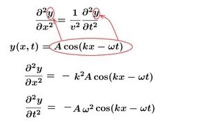
Wave Functions


Intro to Wave Functions
Patrick Ford
Video duration:
8mPlay a video:
Related Videos
Related Practice
 07:31
07:31