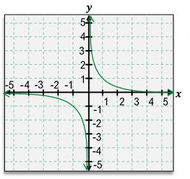
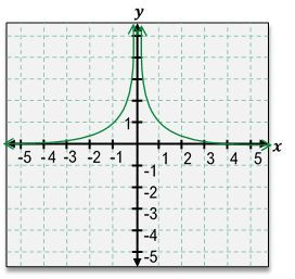
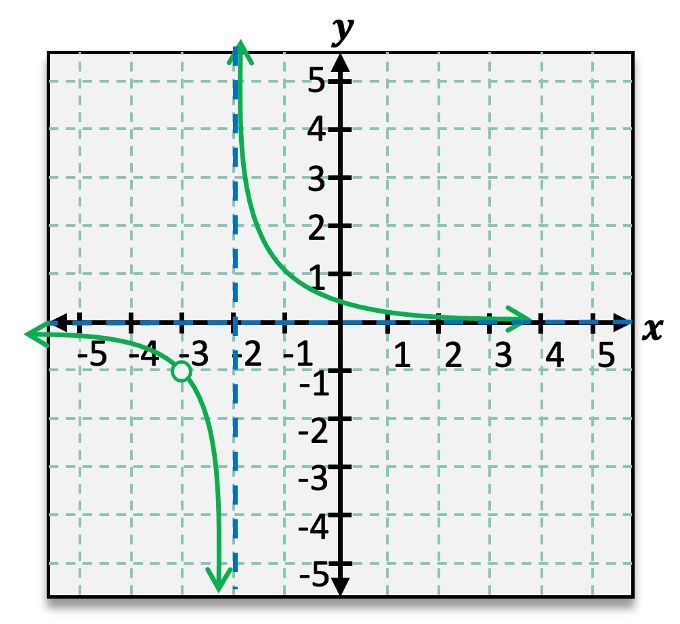
Understanding how to graph rational functions involves recognizing the fundamental components and applying transformations to them. A basic rational function, such as \( f(x) = \frac{1}{x} \), serves as a foundation for more complex graphs. By utilizing transformations, we can manipulate this basic function to create a new graph without performing extensive calculations.
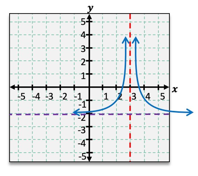
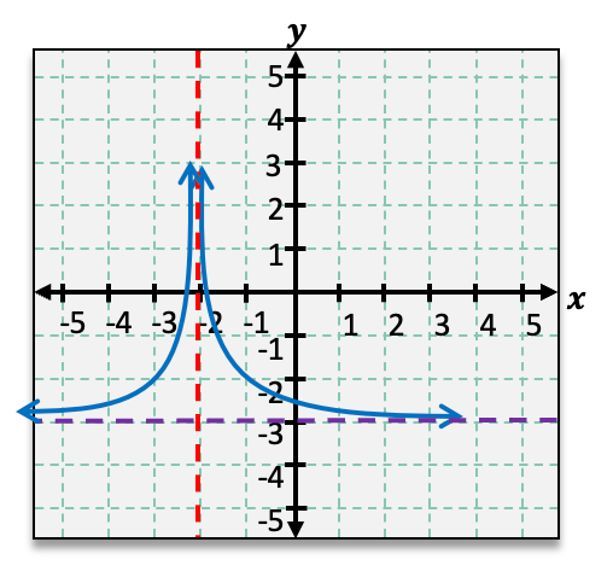
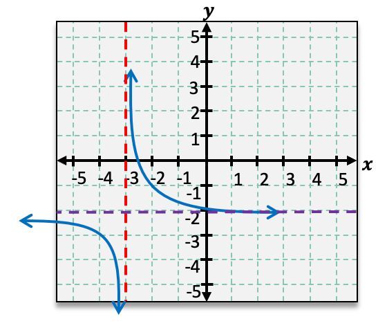
Transformations of rational functions primarily include reflections and shifts. A negative sign outside the function indicates a reflection over the x-axis, while a negative sign inside the function reflects it over the y-axis. Horizontal shifts are represented by \( x - h \), where \( h \) indicates the number of units shifted left or right. Vertical shifts are denoted by \( + k \), indicating movement up or down by \( k \) units.
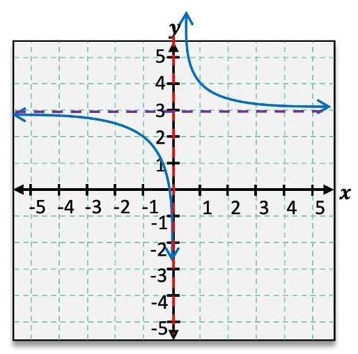
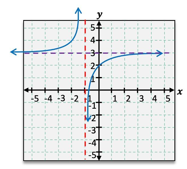
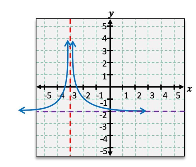
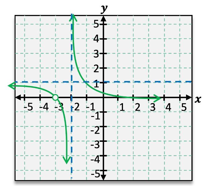
To graph a transformed function, such as \( g(x) = \frac{1}{x - 3} + 1 \), we start by identifying the vertical and horizontal asymptotes. The vertical asymptote is determined by the value of \( h \) in \( x - h \), which in this case is \( x = 3 \). The horizontal asymptote is found from \( k \), leading to \( y = 1 \). These asymptotes are plotted as dashed lines on the graph.
Next, we check for reflections. If there are no negative signs in the function, as in this example, we proceed without reflecting the graph. The next step involves shifting reference points based on the transformations. For instance, the point \( (1, 1) \) shifts 3 units to the right and 1 unit up, resulting in the new point \( (4, 2) \). Similarly, the point \( (-1, -1) \) shifts to \( (2, 0) \).
After plotting the transformed asymptotes and points, we sketch the curves approaching these asymptotes. The resulting graph will resemble the original \( \frac{1}{x} \) graph but will be repositioned according to the transformations applied.
Finally, we analyze the domain and range of the function. The domain is expressed in set notation, indicating intervals where the function is defined. For the function \( g(x) \), the domain is \( (-\infty, 3) \cup (3, \infty) \), reflecting the vertical asymptote at \( x = 3 \). The range follows a similar pattern, resulting in \( (-\infty, 1) \cup (1, \infty) \) due to the horizontal asymptote at \( y = 1 \). Both the domain and range exclude the asymptote values, hence the use of parentheses.
By mastering these transformation techniques, students can effectively graph rational functions and understand their behavior in relation to asymptotes, domain, and range.