Understanding the behavior of polynomial functions involves analyzing various key elements, such as end behavior, x-intercepts, y-intercepts, and turning points. However, to create a complete graph, it is essential to fill in the gaps between these known points. This can be achieved by identifying intervals of unknown behavior and selecting specific x-values within those intervals to calculate corresponding f(x) values.
To begin, break the graph into intervals based on known points. For instance, if you have a known point at x = -2, the interval from negative infinity to -2 represents an area where the behavior of the graph is uncertain. Similarly, you can identify other intervals, such as from -2 to 0, from 0 to 3, and from 3 to positive infinity. Each of these intervals contains unknown behavior that needs to be explored.
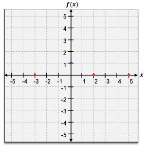
Next, choose x-values within each interval to compute f(x). For the interval from negative infinity to -2, selecting x = -3 is a strategic choice, as it allows for a manageable calculation. For the interval from -2 to 0, x = -1 can be chosen, while for the interval from 0 to 3, x = 2 is appropriate. Finally, for the interval from 3 to infinity, x = 4 can be selected. By calculating f(x) for these chosen x-values, you generate ordered pairs that can be plotted on the graph.
Once you have plotted these points, the next step is to connect them smoothly to visualize the complete behavior of the polynomial function. This process not only provides a clearer picture of the graph but also enhances understanding of how the function behaves across its entire domain. If desired, additional points can be plotted to refine the graph further, ensuring a comprehensive representation of the polynomial function.
In summary, by systematically identifying intervals of unknown behavior and strategically selecting x-values to compute f(x), you can effectively construct a complete graph of a polynomial function, illustrating its overall behavior and characteristics.