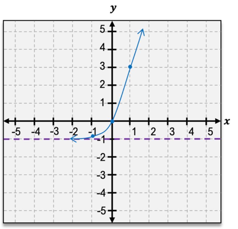
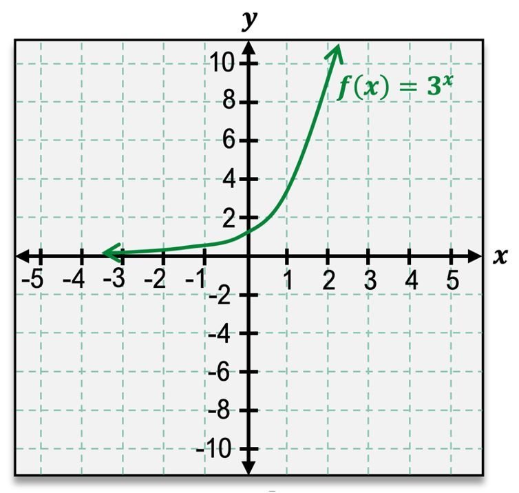
Graphing exponential functions, such as \( f(x) = 2^x \), is a straightforward process compared to polynomial and rational functions. To begin, we can generate ordered pairs by substituting values for \( x \). For instance, when \( x = 0 \), \( f(0) = 2^0 = 1 \), giving us the point (0, 1). Continuing with \( x = 1 \), we find \( f(1) = 2^1 = 2 \), leading to the point (1, 2). As \( x \) increases, the function values grow rapidly: \( f(2) = 4 \), \( f(3) = 8 \), and \( f(10) = 1024 \). This indicates that as \( x \) approaches infinity, \( f(x) \) also approaches infinity, demonstrating the end behavior of the graph.
For negative values of \( x \), we observe that \( f(-1) = 2^{-1} = \frac{1}{2} \) and as \( x \) decreases further, the function values approach zero but never actually reach it. This behavior indicates the presence of a horizontal asymptote at \( y = 0 \), which can be represented by a dashed line on the graph. The graph is continuous, meaning there are no breaks, and it passes the horizontal line test, confirming that it is a one-to-one function.
The overall shape of the graph resembles a stretched lowercase 'e', which can help in visualizing exponential growth. The domain of any exponential function is all real numbers, expressed as \( (-\infty, \infty) \). The range, however, depends on the asymptote; for \( f(x) = 2^x \), the range is \( (0, \infty) \), as the function values are always positive and never touch the asymptote.
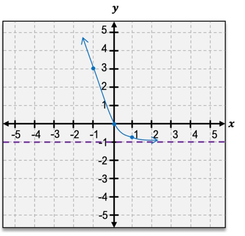
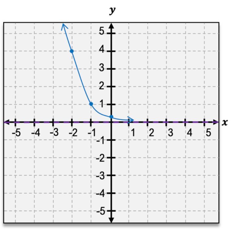
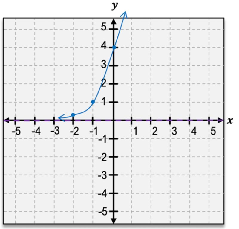
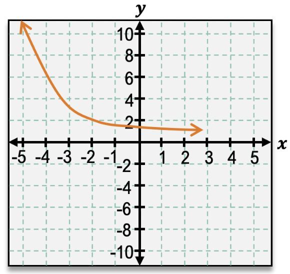
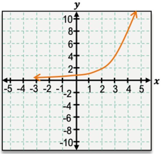
When exploring other exponential functions of the form \( f(x) = b^x \), the base \( b \) significantly influences the graph's behavior. If \( b > 1 \), the graph will always increase, becoming steeper as \( b \) increases (e.g., from \( b = 2 \) to \( b = 5 \)). Conversely, if \( 0 < b < 1 \), the graph will decrease, and it will become steeper as \( b \) approaches zero (e.g., from \( b = \frac{1}{2} \) to \( b = \frac{1}{4} \)). Understanding these characteristics allows for a comprehensive grasp of exponential functions and their graphs.