{Use of Tech} Cell population The ​population ​of a culture of cells after t days is approximated by the function P(t)=1600 / 1 + 7e^−0.02t, for t≥0.
a. Graph the population function.  

Verified step by step guidance

1. Step 1: Understand the function P(t) = \frac{1600}{1 + 7e^{-0.02t}}. This is a logistic function, which is commonly used to model population growth where the growth rate decreases as the population reaches a carrying capacity.
2. Step 2: Identify key features of the logistic function. The carrying capacity, or the maximum population, is 1600. The initial population can be found by evaluating P(0).
3. Step 3: Determine the horizontal asymptotes. As t approaches infinity, the term 7e^{-0.02t} approaches zero, so the function approaches the carrying capacity of 1600. As t approaches negative infinity, the function approaches zero.
4. Step 4: Calculate a few key points to help sketch the graph. Evaluate P(t) at t = 0, t = 10, t = 20, etc., to see how the population changes over time.
5. Step 5: Use a graphing tool or software to plot the function P(t) = \frac{1600}{1 + 7e^{-0.02t}}. Observe the S-shaped curve typical of logistic growth, starting near zero, increasing rapidly, and then leveling off near the carrying capacity.

Key Concepts

Logistic Growth Model

The function P(t) = 1600 / (1 + 7e^(-0.02t)) represents a logistic growth model, which describes how populations grow in a limited environment. Initially, the population grows exponentially, but as resources become limited, the growth rate slows and approaches a maximum carrying capacity, in this case, 1600 cells.

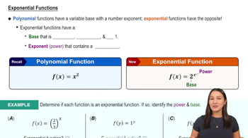
Exponential Function

The term e^(-0.02t) in the population function indicates an exponential decay factor, which influences how quickly the population approaches its carrying capacity. Exponential functions are characterized by their rapid growth or decay, and in this context, they help model the initial growth phase of the cell population before it stabilizes.

Graphing Functions

Graphing the population function involves plotting the values of P(t) against t to visualize how the cell population changes over time. Understanding how to graph functions is essential in calculus, as it allows for the analysis of behavior, trends, and key features such as intercepts, asymptotes, and limits.