U.S. population growth The population p(t) (in millions) of the United States t years after the year 1900 is shown in the figure. Approximately when (in what year) was the U.S. population growing most slowly between 1925 and 2020? Estimate the growth rate in that year. <IMAGE>
Table of contents
- 0. Functions7h 55m
- Introduction to Functions18m
- Piecewise Functions10m
- Properties of Functions9m
- Common Functions1h 8m
- Transformations5m
- Combining Functions27m
- Exponent rules32m
- Exponential Functions28m
- Logarithmic Functions24m
- Properties of Logarithms36m
- Exponential & Logarithmic Equations35m
- Introduction to Trigonometric Functions38m
- Graphs of Trigonometric Functions44m
- Trigonometric Identities47m
- Inverse Trigonometric Functions48m
- 1. Limits and Continuity2h 2m
- 2. Intro to Derivatives1h 33m
- 3. Techniques of Differentiation3h 18m
- 4. Applications of Derivatives2h 38m
- 5. Graphical Applications of Derivatives6h 2m
- 6. Derivatives of Inverse, Exponential, & Logarithmic Functions2h 37m
- 7. Antiderivatives & Indefinite Integrals1h 26m
- 8. Definite Integrals4h 44m
- 9. Graphical Applications of Integrals2h 27m
- 10. Physics Applications of Integrals 3h 16m
- 11. Integrals of Inverse, Exponential, & Logarithmic Functions2h 31m
- 12. Techniques of Integration7h 41m
- 13. Intro to Differential Equations2h 55m
- 14. Sequences & Series5h 36m
- 15. Power Series2h 19m
- 16. Parametric Equations & Polar Coordinates7h 58m
2. Intro to Derivatives
Tangent Lines and Derivatives
Problem 97
Textbook Question
97–100. Logistic growth Scientists often use the logistic growth function P(t) = P₀K / P₀+(K−P₀)e^−r₀t to model population growth, where P₀ is the initial population at time t=0, K is the carrying capacity, and r₀ is the base growth rate. The carrying capacity is a theoretical upper bound on the total population that the surrounding environment can support. The figure shows the sigmoid (S-shaped) curve associated with a typical logistic model. <IMAGE>
{Use of Tech} Gone fishing When a reservoir is created by a new dam, 50 fish are introduced into the reservoir, which has an estimated carrying capacity of 8000 fish. A logistic model of the fish population is P(t) = 400,000 / 50+7950e^−0.5t, where t is measured in years.
a. Graph P using a graphing utility. Experiment with different windows until you produce an S-shaped curve characteristic of the logistic model. What window works well for this function?
 Verified step by step guidance
1
Understand the logistic growth function: P(t) = \(\frac{P_0 K}{P_0 + (K - P_0) e^{-r_0 t}\)}, where P_0 is the initial population, K is the carrying capacity, and r_0 is the growth rate.
Identify the parameters from the problem: P_0 = 50 (initial fish population), K = 8000 (carrying capacity), and r_0 = 0.5 (growth rate). The logistic model given is P(t) = \(\frac{400,000}{50 + 7950 e^{-0.5t}\)}.
To graph the function, use a graphing utility. Input the function P(t) = \(\frac{400,000}{50 + 7950 e^{-0.5t}\)} into the graphing tool.
Experiment with different window settings to capture the S-shaped curve. A good starting point for the window might be: x-axis (time, t) from 0 to 20 years, and y-axis (population, P(t)) from 0 to 9000 fish.
Adjust the window settings as needed to ensure the entire S-shaped curve is visible, showing the initial growth, the inflection point, and the leveling off as the population approaches the carrying capacity.
 Verified video answer for a similar problem:
This video solution was recommended by our tutors as helpful for the problem above
Video duration:
5mPlay a video:
0 Comments
Key Concepts
Here are the essential concepts you must grasp in order to answer the question correctly.
Logistic Growth Function
The logistic growth function models population growth that is initially exponential but slows as the population approaches a maximum limit, known as the carrying capacity (K). The function is represented as P(t) = P₀K / (P₀ + (K - P₀)e^(-r₀t)), where P₀ is the initial population, r₀ is the growth rate, and t is time. This model is crucial for understanding how populations grow in constrained environments.
Recommended video:

Derivative of the Natural Logarithmic Function Example 7
Carrying Capacity
Carrying capacity (K) refers to the maximum population size that an environment can sustain indefinitely without being degraded. It is a critical concept in ecology and population dynamics, as it influences the growth rate and stability of populations. In the context of the logistic model, as the population approaches K, the growth rate decreases, leading to a leveling off of the population size.
Recommended video:

Intro to the Chain Rule Example 2
Graphing Logistic Functions
Graphing logistic functions involves plotting the population over time to visualize its growth pattern, which typically forms an S-shaped curve. This curve illustrates the initial rapid growth phase, followed by a slowdown as the population nears the carrying capacity. Understanding how to adjust the graphing window is essential for accurately displaying the behavior of the logistic model and identifying key features such as inflection points.
Recommended video:

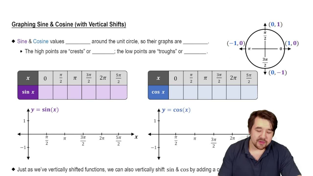
Graph of Sine and Cosine Function
Related Videos
Related Practice
Textbook Question
239
views


