{Use of Tech} A different interpretation of marginal cost Supp...

Question

{Use of Tech} A different interpretation of marginal cost Suppose a large company makes 25,000 gadgets per year in batches of x items at a time. After analyzing setup costs to produce each batch and taking into account storage costs, planners have determined that the total cost C(x) of producing 25,000 gadgets in batches of x items at a time is given by C(x) = 1,250,000+125,000,000 / x + 1.5x.
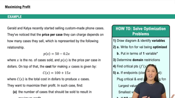
a. Determine the marginal cost and average cost functions. Graph and interpret these functions.

a. Determine the marginal cost and average cost functions. Graph and interpret these functions.

Accepted Answer

Hello. In this video, we are going to be solving for an average cost and a marginal cost. So we are told that a factory produces 50,000 units of product each year in lots of X units. After considering the setup and storage costs, the total cost function of producing 50,000 units in lots of X units is given by T X equal to 2 million plus 150 million divided by X plus 3X. We want to find the marginal cost and average cost functions. Then we want to graph these functions using a utility and provide an interpretation of them. So, let's go ahead and start by finding the average cost. Now, in order to find the average cost, what we are trying to find is the average cost of all the units produced in one year. Recall that the problem tells us that the factory produces 50,000 units each year. And since the function that determines the production of these units is given by T X, in order to solve for the average function or average cost, we are going to take the function T of X and divide it by the total amount of units produced each year, which is 50,000. So, again, T X is 2 million plus 150 million divided by X plus 3 X. So, our average cost will be this function, which is 2 million. Plus 150 million. Divided by X plus 3 X. And this will all be divided by 50,000. Now, after algebraic simplification, we can further simplify this function to be 40. Plus 3000 Divided by X. Plus 3 divided. By 50,000 multiplied by X. And this is going to be the function that represents the average cost of producing the 50,000 units yearly. Now what we want to go ahead and do is you want to go ahead and solve for the marginal cost. Now, in order to solve for the marginal cost, what we want to do is you want to take the derivative of the given function. So, again, our function is T X. Equal to 2 million. Plus 150 million. Divided by X plus 3 X. What we are going to do is we're going to take the derivative of this function. So, taking the derivative with respect to X, we will go ahead and take the derivative of each term respectively. Now 2 million is a constant value, and the derivative of any constant will be zero, so the derivative of the first term is 0. Now, for the second term, we have X in the denominator, which means that we will need to use the quotient rule. After applying the quotient rule. The derivative of the second term will be negative. 150 million. Divided by X2. And for the final term, we will take the derivative by using the power rule, and the derivative of 3 X will just be 3. So, this simplifies the function to be T X equal to -150 million. Divided by X2 + 3. This is going to be the function that represents the marginal cost. Now that we have the functions for the marginal cost and for the average cost, we will go ahead and use a graphing utility to plot these two functions. So, what I have here is the plot of both of the functions on the same axis. Now, let's go ahead and provide an interpretation. We will start with the interpretation for the average cost. Now notice that the average cost starts off high in the X axis in the Y axis, and slowly decreases towards the X-axis, stabilizing around, let's say, Y is equal to approximately 40. What this means is that in terms of the average cost, The average cost decreases as the amount of units increase. So, Average cost. Will decrease. To $40. As The amount of units. Increase So that is the interpretation of the average cost graph. But now, what about the marginal cost? Well, since the marginal cost slowly decreases or increases as it slowly increases as the value of X increases, that means marginal cost. Will increase As the amount of units increase. And this is going to be the interpretation of the given graph. So I hope this video helps you in understanding on how to approach this problem, and I will go ahead and see you all in the next video.

Key Concepts

Marginal Cost

Average Cost

Graphing Functions

Watch next