Skip to main content
Calculus
My Course
Learn
Exam Prep
AI Tutor
Study Guides
Textbook Solutions
Flashcards
Explore
Try the app
My Course
Learn
Exam Prep
AI Tutor
Study Guides
Textbook Solutions
Flashcards
Explore
Try the app
?
Select textbook and Institution
Improve your experience by picking them
Table of contents
Skip topic navigation
0. Functions
7h 55m
Chapter worksheet
Introduction to Functions
18m
Piecewise Functions
10m
Properties of Functions
9m
Common Functions
1h 8m
Transformations
5m
Combining Functions
27m
Exponent rules
32m
Exponential Functions
28m
Logarithmic Functions
24m
Properties of Logarithms
36m
Exponential & Logarithmic Equations
35m
Introduction to Trigonometric Functions
38m
Graphs of Trigonometric Functions
44m
Trigonometric Identities
47m
Inverse Trigonometric Functions
48m
1. Limits and Continuity
2h 2m
Chapter worksheet
Introduction to Limits
41m
Finding Limits Algebraically
40m
Continuity
40m
2. Intro to Derivatives
1h 33m
Chapter worksheet
Tangent Lines and Derivatives
30m
Derivatives as Functions
14m
Basic Graphing of the Derivative
23m
Differentiability
26m
3. Techniques of Differentiation
3h 18m
Chapter worksheet
Basic Rules of Differentiation
39m
Higher Order Derivatives
12m
Product and Quotient Rules
55m
Derivatives of Trig Functions
40m
The Chain Rule
49m
4. Applications of Derivatives
2h 38m
Chapter worksheet
Motion Analysis
36m
Implicit Differentiation
27m
Related Rates
59m
Linearization
13m
Differentials
21m
5. Graphical Applications of Derivatives
6h 2m
Chapter worksheet
Intro to Extrema
23m
Finding Global Extrema
50m
The First Derivative Test
1h 5m
Concavity
1h 1m
The Second Derivative Test
31m
Curve Sketching
44m
Applied Optimization
1h 25m
6. Derivatives of Inverse, Exponential, & Logarithmic Functions
2h 37m
Chapter worksheet
Derivatives of Exponential & Logarithmic Functions
1h 52m
Logarithmic Differentiation
20m
Derivatives of Inverse Trigonometric Functions
24m
7. Antiderivatives & Indefinite Integrals
1h 26m
Chapter worksheet
Antiderivatives
17m
Indefinite Integrals
25m
Integrals of Trig Functions
15m
Initial Value Problems
27m
8. Definite Integrals
4h 44m
Chapter worksheet
Estimating Area with Finite Sums
42m
Riemann Sums
1h 21m
Introduction to Definite Integrals
22m
Fundamental Theorem of Calculus
37m
Average Value of a Function
21m
Substitution
1h 19m
9. Graphical Applications of Integrals
2h 27m
Chapter worksheet
Area Between Curves
1h 18m
Introduction to Volume & Disk Method
1h 8m
10. Physics Applications of Integrals
3h 16m
Chapter worksheet
Kinematics
1h 13m
Work
2h 3m
11. Integrals of Inverse, Exponential, & Logarithmic Functions
2h 31m
Chapter worksheet
Integrals of Exponential Functions
40m
Integrals Involving Logarithmic Functions
58m
Integrals Involving Inverse Trigonometric Functions
52m
12. Techniques of Integration
7h 41m
Chapter worksheet
Integration by Parts
2h 32m
Partial Fractions
4h 29m
Improper Integrals
39m
13. Intro to Differential Equations
2h 55m
Chapter worksheet
Basics of Differential Equations
48m
Slope Fields
19m
Euler's Method
22m
Separable Differential Equations
1h 25m
14. Sequences & Series
5h 36m
Chapter worksheet
Sequences
1h 22m
Review of Factorials
11m
Series
44m
Convergence Tests
3h 17m
15. Power Series
2h 19m
Chapter worksheet
Introduction to Power Series
1h 9m
Taylor Series & Taylor Polynomials
1h 10m
16. Parametric Equations & Polar Coordinates
7h 58m
Chapter worksheet
Parametric Equations
1h 6m
Calculus with Parametric Curves
1h 13m
Polar Coordinates
2h 5m
Calculus in Polar Coordinates
55m
Conic Sections
2h 36m
0. Functions
Graphs of Trigonometric Functions
Calculus
0. Functions
Graphs of Trigonometric Functions
Previous video
Next video
Struggling with Calculus?
Join thousands of students who trust us to help them ace their exams!
Watch the first video
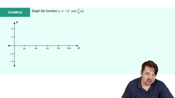
Introduction to Cotangent Graph
Nick
Video duration:
5m
Play a video:
Previous video
Next video
Related Videos
Related Practice
5:53
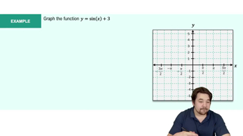
Graph of Sine and Cosine Function
1174
views
27
rank
2:18
Graph of Sine and Cosine Function Example 1
702
views
12
rank
6:22
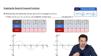
Graphs of Secant and Cosecant Functions
770
views
21
rank
5:43
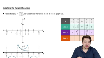
Introduction to Tangent Graph
598
views
8
rank
3:15
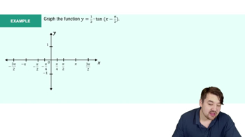
Introduction to Tangent Graph Example 1
509
views
9
rank
1
comments
3:40
Introduction to Cotangent Graph Example 1
437
views
9
rank
Show more videos


 5:53
5:53