Local max/min of x¹⸍ˣ Use analytical methods to find all local extrema of the function ƒ(x) = x¹⸍ˣ , for x > 0 . Verify your work using a graphing utility.

Verified step by step guidance

1. To find the local extrema of the function \( f(x) = x^{1/x} \), first take the derivative of the function with respect to \( x \). This involves using the chain rule and the power rule.
2. Express \( f(x) = x^{1/x} \) as \( f(x) = e^{(1/x) \ln(x)} \) to facilitate differentiation. Differentiate \( f(x) = e^{(1/x) \ln(x)} \) using the chain rule: \( f'(x) = e^{(1/x) \ln(x)} \cdot \left( \frac{d}{dx} \left( \frac{\ln(x)}{x} \right) \right) \).
3. Calculate \( \frac{d}{dx} \left( \frac{\ln(x)}{x} \right) \) using the quotient rule: \( \frac{d}{dx} \left( \frac{\ln(x)}{x} \right) = \frac{x \cdot \frac{1}{x} - \ln(x) \cdot 1}{x^2} = \frac{1 - \ln(x)}{x^2} \).
4. Set \( f'(x) = 0 \) to find critical points: \( e^{(1/x) \ln(x)} \cdot \frac{1 - \ln(x)}{x^2} = 0 \). Since \( e^{(1/x) \ln(x)} \neq 0 \), solve \( \frac{1 - \ln(x)}{x^2} = 0 \), which simplifies to \( 1 - \ln(x) = 0 \). Therefore, \( \ln(x) = 1 \), giving \( x = e \).
5. Verify the nature of the critical point \( x = e \) by using the second derivative test or by analyzing the sign changes of \( f'(x) \) around \( x = e \). This will confirm whether \( x = e \) is a local maximum or minimum. Finally, use a graphing utility to visualize the function and confirm the analytical results.

Key Concepts

Critical Points

Critical points of a function occur where its derivative is zero or undefined. These points are essential for finding local maxima and minima, as they indicate where the function's slope changes. To find critical points, we first compute the derivative of the function and solve for x when the derivative equals zero.

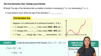
First Derivative Test

The First Derivative Test is a method used to determine whether a critical point is a local maximum, local minimum, or neither. By analyzing the sign of the derivative before and after the critical point, we can conclude if the function is increasing or decreasing. If the derivative changes from positive to negative, the point is a local maximum; if it changes from negative to positive, it is a local minimum.

Graphing Utility Verification

Using a graphing utility allows for visual confirmation of the analytical results obtained from calculus. By plotting the function, one can observe the behavior of the graph around the critical points, confirming the presence of local maxima and minima. This visual approach helps to validate the findings from the derivative tests and provides insight into the function's overall shape.