2. Intro to Derivatives
Tangent Lines and Derivatives
Problem 99b
Textbook Question
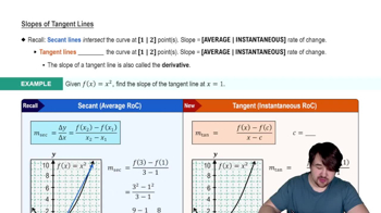
The population of the United States (in millions) by decade is given in the table, where t is the number of years after 1910. These data are plotted and fitted with a smooth curve y = p(t) in the figure. <IMAGE><IMAGE>
Explain why the average rate of growth from 1950 to 1960 is a good approximation to the (instantaneous) rate of growth in 1955.
 Verified step by step guidance
1
To understand why the average rate of growth from 1950 to 1960 is a good approximation to the instantaneous rate of growth in 1955, we need to consider the concept of average rate of change and instantaneous rate of change. The average rate of change of a function over an interval [a, b] is given by the formula: \( \frac{p(b) - p(a)}{b - a} \), where p(t) is the population function.
In this context, the average rate of growth from 1950 to 1960 is calculated using the population values at t = 40 (1950) and t = 50 (1960). This gives us the average rate of change over the decade.
The instantaneous rate of change at a specific point, such as 1955, is represented by the derivative of the function p(t) at that point, denoted as p'(t). This derivative gives the slope of the tangent line to the curve at t = 45 (1955).
If the function p(t) is smooth and does not have any abrupt changes in its slope over the interval from 1950 to 1960, the average rate of change over this interval will be close to the instantaneous rate of change at the midpoint of the interval, which is 1955.
Therefore, if the curve is relatively linear or smoothly varying between 1950 and 1960, the average rate of growth from 1950 to 1960 serves as a good approximation for the instantaneous rate of growth in 1955, because the average rate captures the overall trend of the function over that period.
Verified video answer for a similar problem:This video solution was recommended by our tutors as helpful for the problem above
Video duration:
3mWas this helpful?
Key Concepts
Here are the essential concepts you must grasp in order to answer the question correctly.
Average Rate of Change
The average rate of change of a function over an interval measures how much the function's value changes per unit of input over that interval. It is calculated as the difference in the function's values at the endpoints of the interval divided by the difference in the input values. In this context, it provides a general idea of how the population grew from 1950 to 1960.
Recommended video:

 06:37
06:37Average Value of a Function
Instantaneous Rate of Change
The instantaneous rate of change of a function at a specific point is the limit of the average rate of change as the interval approaches zero. It is represented mathematically by the derivative of the function at that point. In this case, it reflects the population growth rate precisely at the year 1955.
Recommended video:
 04:16
04:16Intro To Related Rates
Smooth Curve Fitting
Smooth curve fitting involves creating a continuous function that closely approximates a set of data points. This technique helps in understanding trends and making predictions. The fitted curve in the population data allows us to estimate both average and instantaneous rates of growth, making it easier to analyze changes over time.
Recommended video:
 11:41
11:41Summary of Curve Sketching
 5:13m
5:13mWatch next
Master Slopes of Tangent Lines with a bite sized video explanation from Nick
Start learningRelated Videos
Related Practice