Graphing functions Sketch a graph of each function.

...

Question

Graphing functions Sketch a graph of each function.

g(x) = { 4-2x if x ≤ 1 , (x-1)² + 2 if x > 1

Accepted Answer

Hello there. Today we're gonna solve the following practice problem together. So first off, let us read the problem and highlight all the key pieces of information that we need to use in order to solve this problem. Consider the piece-wise function H of X is equal to curly bracket of 3 minus X + 1 to the power of 2. If X is less than or equal to 2. And 2 X minus 10 if X is greater than 2, plot the graph of the function. So it appears for this particular prompt, what we're ultimately trying to do is we're trying to create a graph of this piecewise function for HF X. So now that we know that we're trying to create a graph for this piece-wise function of HFX. Let us first start by breaking up our piece-wise function into two separate pieces and solve for them individually means these will produce two separate curves, and then we need to combine the curves into one graph to represent the graph with the piece-wise function. So let us start with our first function, which is 3 minus X + 1 to the power of 2. So once again, we're focusing our attention on the first piece, so we're focusing once again on. 3 Minus X + 1. And this will be to the power of 2, and this is for the condition where once again that X is less than or equal to 2. Fantastic. So, we need to note, if you, you can automatically, like there's two separate, I'll take a moment here to pause briefly. There's two different ways you can plot this graph. So you can take each individual piece, these two separate functions, and you can each graph them separately by hand or sketch them separately. By hand or you can go ahead and take both of these functions and plug them straight into some graphing software of your choice, and it will automatically put it into one big combined graph. But what I'm gonna do is we're just going to solve for all the. Little like we're trying to solve for coordinate points separately, so we're gonna start with our first function and then look at our second function, and we're trying to figure out what our needed coordinate points are to help us produce the graphs, but if you just want to go ahead and Take these two functions and plugging in and plug them into some graphing software and just get the graph all in one go, you could totally do that because it doesn't specify in the prom itself whether or not we are asked to graph it by hand or to just use graphing software. So going back now, so right now, like I mentioned, we're trying to figure out for our first piece of our of our piece wise function, we're trying to figure out the coordinate points. So looking at this expression because we have this power of 2 here, we should be thinking oh we might. be dealing with a parabola. So because of that knowledge, when you ultimately, when we graph this, we will discover that this is a downward opening parabola, and it will have a vertex point which will write this in green, V for vertex. The vertex will be at -1, instead of using equal senses do. On here, so the vertex V for this parabola will be at -13, and once again, note that this is our coordinate point, which is for X.Y. So this is -1.3, so that's our vertex. And now we need to figure out the points that we're going to need to plot this particular function, this particular curve. So in order to plot some points, we need to find a few separate coordinate points in order to do that. We need to just take different values for X and plug it into our function to solve for our different coordinate points. So for example, when X is equal to 0, we will find that H of X is going to be equal to 3 minus 0. Plus 1 to the power 2, which will be equal to 2. And once again, this is noting that we have to note that X is less than or equal to 2. So when 0 is less than 2, and then we could also use X is equal to 2 because X is less than or equal to 2. So when X is equal to 2, H of X is going to be equal to 3 minus. 2 + 1 to 2, and then this will be equal to -6. Fantastic. So now we could sketch our parabola from the vertex, which once again is -1.3, and then it will have to pass through the points, and let's write this down, this is important. You'll have to pass through the points 0.2. And it will also have to pass through the points 2, -6. And also we need to note that it stops at. So it stops at X equals 2. Awesome. So, moving right along here, so right now, before we graph everything, I'm just basically we're creating the backbone that we need to graph a graph. So right now we're doing all of the math to help us properly plot our graph at large here. So, moving on to our next step, and let's put a, let's put a line. Between it. So now this is our that's for our first function. So now let's switch gears to focus on our second function here. So right now we need to plot the second piece, so let us note that for our second piece, this will be for, once again, 2 X minus 10. And let's note that for this particular one, so this is 2 X minus 10, and this is for the condition where X is greater than 2. Fantastic. So, With that in mind, using the similar methodology like we did for our previous piece, we need to note for this one, since looking at the formatting of the function as it is, we will be dealing with a straight line, as we should recall, and this straight line will have a slope of 2. So let's make a note of this. So S for slope is equal to 2. And we need to note that there will be a Y. Intercept At so this will be a y intercept at -10 fantastic. And in order to plot like we did before, we need to find two points on the line at which the conditions X is greater than 2 is met. So for example, like we did previously, we could plug in different values for X. So in this case, we know that 3 is greater than 2, so let's use X is equal. 3, and when X is equal to 3, that will mean that H of X, so instead of rewriting the entire function again, I'm just going to write the answer. So when you plug in a value for 3 into our function for H of X is equal to 2 x minus 10, we will find that it's equal to -4. And similarly, if we use X is equal to 4, we will find that H of X is equal to once again. So then once again, so this is where when we plug in a value of 4 in for X, we will find that it's ultimately equal to -2. Fantastic. So, now we need to draw our line and it will need to pass through the points. Once again, we'll pass through the points 34, and it will also need to pass through the points 42. And it will be extending, so let's make a note of this. So this will be E for extending, will be extending. To the right, so extending to the right, which I'll put an R in quotation marks, so. The quotation marks around E, so that means extending, so it's extending to the right. Fantastic. So, now that we have all the information we need to point, like to plot our graphs, let us create a graph for each of our, so well, what I'm gonna do is I plugged in. Our piece-wise function into some graphing software, and I created the three graphs shown. So going for our first graph, so let's make a note of this. So let's call our first graph, which will be our first piece, which is for, once again, 3 minus X + 1 to the power 2, it will be our parabola, and as you can see, we have our parabola. That's at the points -1, 3, and at 0.2 and our once again it will stop at X equals 2, so we have a 2.6, so that's our first graph. And then our second graph. Which is for our second piece, which is for 2 X minus 10, we have our two different points that our line crosses through, which is 3.4 and 4.2, and it also intersects the X axis at 5.0. And when you combine both graphs together, so this is 1 + 2, we get our final graph, which this is our final answer. I'll let's put a green box around it because this is our final graph. This is what our final answer will have to look like for our graph for the piece wise function. And as you can see, we basically connect the two graphs, so where the parabola ends at 0.2.6, that's where our second piece connects and extends to the right. Which once again this will be, it's basically where our parabola ends at 2.6. Our second piece will begin from that point extending to the right. And that is it. We've officially solved for this problem. Thank you so much for watching. Hopefully that helped, and I can't wait to see you in the next video. Bye.

Graphing functions Sketch a graph of each function.

g(x) = { 4-2x if x ≤ 1 , (x-1)² + 2 if x > 1

Key Concepts

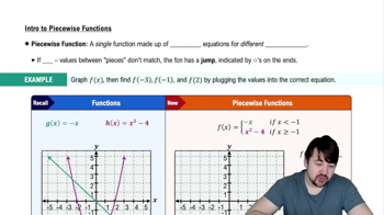
Piecewise Functions

Graphing Techniques

Continuity and Discontinuity

Watch next