Ch. 2 - Limits and Continuity
Hass - Thomas' Calculus 15th Edition
Hass15th EditionThomas' CalculusISBN: 9780137616077Not the one you use?Change textbook
Chapter 2, Problem 2.5.72

Use the Intermediate Value Theorem in Exercises 69–74 to prove that each equation has a solution. Then use a graphing calculator or computer grapher to solve the equations.
x³ − 15x + 1 = 0 (three roots)

Verified step by step guidance
1
Understand the Intermediate Value Theorem (IVT): It states that if a continuous function f(x) takes on values of opposite signs at two points a and b, then there exists at least one c in the interval (a, b) such that f(c) = 0.
Identify the function: Here, the function is f(x) = x³ − 15x + 1. This is a polynomial function, which is continuous everywhere.
Choose appropriate intervals: To apply the IVT, we need to find intervals where the function changes sign. Start by evaluating f(x) at various points to find intervals where f(x) changes from positive to negative or vice versa.
Evaluate the function at chosen points: Calculate f(x) at several points, such as f(-3), f(0), f(3), etc., to find intervals where the sign changes. For example, if f(-3) < 0 and f(0) > 0, then there is a root in the interval (-3, 0). Repeat this process to find all intervals where the function changes sign.
Use a graphing calculator or computer grapher: Once you have identified the intervals using the IVT, use a graphing tool to visualize the function and find the approximate values of the roots within those intervals.

Verified video answer for a similar problem:

This video solution was recommended by our tutors as helpful for the problem above.
Video duration:
2m
Was this helpful?

Key Concepts

Here are the essential concepts you must grasp in order to answer the question correctly.

Intermediate Value Theorem

The Intermediate Value Theorem states that if a function is continuous on a closed interval [a, b] and takes on different signs at the endpoints (f(a) and f(b)), then there exists at least one c in (a, b) such that f(c) = 0. This theorem is fundamental for proving the existence of roots in continuous functions.
Recommended video:
06:11
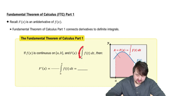
Fundamental Theorem of Calculus Part 1

Continuous Functions

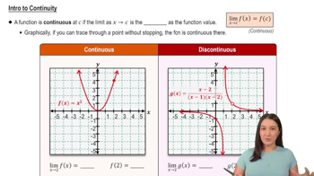
A continuous function is one where small changes in the input result in small changes in the output. Formally, a function f is continuous at a point x = c if the limit of f as x approaches c equals f(c). Understanding continuity is crucial for applying the Intermediate Value Theorem effectively.
Recommended video:
05:34
Intro to Continuity

Graphing Techniques

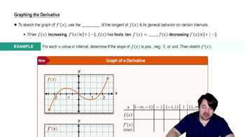
Graphing techniques involve using tools like graphing calculators or software to visualize functions. By plotting the function, one can identify where it crosses the x-axis, indicating the roots of the equation. This visual approach complements analytical methods like the Intermediate Value Theorem in finding solutions.
Recommended video:
06:15
Graphing The Derivative