Shifting Lineweaver-Burk Plots - Online Tutor, Practice Problems & Exam Prep

The Lineweaver-Burk plot, a double reciprocal plot, visualizes enzyme kinetics by plotting the reciprocal of substrate concentration on the x-axis and the reciprocal of initial reaction velocity (v₀) on the y-axis. The slope, defined as the ratio of K_m to V_max, is always positive, indicating that K_m and V_max increase towards zero. Understanding these relationships is crucial for analyzing enzyme behavior, especially in the context of competitive inhibition and other regulatory mechanisms.

Shifting Lineweaver-Burk Plots

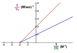
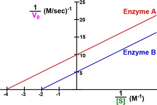
In this video, we're going to talk even more details about a Lineweaver-Burk plot, specifically how to shift the line on a Lineweaver-Burk plot. So recall from our previous lesson videos that the Lineweaver-Burk equation resembles the equation of a line. And so what this means is that we can take the equation of a line, which is y=mx+b, and substitute in enzyme kinetics variables to get the Lineweaver-Burk equation. And so when it comes down to it, what actually defines a line are 2 different factors. The first factor that defines a line is the slope of the line or the m variable in the equation of the line, or the KV_max ratio in the Lineweaver-Burk equation. And the second factor that defines a line is actually the y-intercept of the line, which is the variable b in the equation of the line and the reciprocal of the V_max in the Lineweaver-Burk equation.

And so if we start off with just talking about the slope of the line, recall from your previous courses that when the slope of the line is equal to 0, that means that the line is going to be completely horizontal. It's going to be a completely horizontal line when the slope is equal to 0. And as we begin to increase the slope, as we begin to increase the value of the slope, that will make the line become a steeper line. So that will make the line steeper. And so if we take a look at this Lineweaver-Burk plot that we have down below, notice that this horizontal red line that we see here, as we set up above, horizontal lines will have a slope or, that is going to be equal to 0. So we know that the slope of this red line, or the m value, is going to be equal to 0. And also, as we said up above, if we increase the value of the slope, that's going to make the line steeper. So notice that this green line right here is much steeper and so that means that its slope must be greater than the value 0.

And so, essentially what you'll notice is that the slope is also going to be equal to the rise over the run. And so if we wanted to determine the slope of this green line right here, all we would need to do is start at any point on the line and figure out how much do we need to rise or how much do we need to go up and how much do we need to go, to the right or how much do we need to run horizontally in order to, get back to a point on our line. And so, if we start at this point, we can see that we need to go up 1 unit and to the right one unit in order to get to a point on our line, which means that the rise is going to be 1 and the run will also be 1, and of course 11 is just 1. And so that means that the slope of this line is just going to be 1.

And so, what we can see is that a line that has a slope of 0 is going to be horizontal and if we increase the value of the slope, then we're just going to get ourselves a steeper line, as we see here. Now, if we were to increase the value of the slope to 2, then here we would have a steeper line, and if we were to increase the value of the slope to 3, then we would have an even steeper line. So you can see the effect that increasing the slope will have on the steepness of the line.

Now moving on to the y-intercept, the y-intercept b, increasing the value of the y-intercept is actually going to elevate, it's going to elevate the position that the line intersects the y-axis. So remember that the y-intercept is going to be the value of y when it crosses the y-axis, which is going to be this horizontal axis. So now notice looking at this Lineweaver-Burk plot here in the middle, we have a horizontal line, so we already know that horizontal lines are going to have a slope equal to 0. So we can go ahead and say that the slope is equal to 0 here. However, notice that this horizontal line is crossing the y-axis at a different position than the horizontal line that we had over here. Notice that the horizontal line on the left is crossing the y-axis specifically at the value of 1. However, over here on the right, this horizontal line is crossing the y-axis at a different position at a value of 2. And so what this shows is that if we increase the value of the y-intercept b, that's going to elevate the position of where the line is going to intersect the y-axis.

And so essentially when it comes to shifting the line on a Lineweaver-Burk plot, all we need to consider is the slope of the line and the y-intercept of the line. Now, the last point that I want to make, that's important about shifting the lines of a Lineweaver-Burk plot is that the slope of a line on a Lineweaver-Burk plot, which is of course going to be, the m which is going to be the ratio of the K over the V_max. So we can say that the slope, which is K over V_max, cannot actually be 0 or have a negative value. So essentially what this means is that for Lineweaver-Burk plots, we're never going to see a Lineweaver-Burk plot where we have a slope of 0. So we're never going to see horizontal lines like this, and we're also never going to see a slope that has a negative value. So we're never going to see lines that go in this direction and decrease from left to right. So what we can say is that the slope, which is the K of the V_max, is never going to be negative and it's never going to be 0. It's always going to have some kind of value. And so, essentially we will always expect the lines of our Lineweaver-Burk plot to have a positive value and have a positive slope. And so that makes it a little bit easier to interpret as well and it takes away a lot fewer factors that we need to worry about.

This concludes our lesson on shifting Lineweaver-Burk plots by using the slope of the line and the y-intercept of a line. In our next lesson video, we're going to talk about how to quickly look and visualize a Lineweaver-Burk plot and analyze the kilometers and the V_max. So I'll see you guys in that lesson video.

Shifting Lineweaver-Burk Plots

In this video, we're going to talk about how to glance at lines on a Lineweaver-Burk plot and quickly visualize whether there have been increases or decreases to the Kilometers and or the v max. And so this will be a skill that will be especially useful to you guys once we start talking about enzyme inhibitors later in our course. Now, I also want to point out that in this video, you might get a little bit confused because we're going to talk about some counterintuitive stuff. But if you do get confused, hang on tight because in our next example video, I'm going to show you guys an example of how to apply this counterintuitive stuff, so hopefully things will start clicking and it'll make a lot more sense to you guys after our next example video.

Let's go on and get started here. First, I want you guys to recall from our previous lesson videos that a Lineweaver-Burk plot is also known as a double reciprocal plot because it plots reciprocals on the x and the y axis. On the x-axis, it plots the reciprocal of the substrate concentration, and on the y-axis, it plots the reciprocal of the initial reaction velocity or v₀. Because both the x and the y axes in a Lineweaver-Burk plot are actually reciprocals, essentially one over the substrate concentration and one over the initial reaction velocity v₀, we can say that the substrate concentration and the initial reaction velocity themselves will actually increase towards 0. That's right. I said increase, not decrease towards 0, which is a little counterintuitive.

Let's take a look at our image down below to begin clearing up some of this counterintuitive stuff. In this Lineweaver-Burk plot down below, we're first going to focus only on the x-axis and we're going to kind of ignore the y-axis for a little while. Notice that the x-axis plots the reciprocal of the substrate concentration, and normally on either side of this 0 on the x-axis, we expect the magnitude on the right side of the x-axis to increase towards the right in that direction. And on the left side of the 0 on the x-axis, we expect the magnitude to increase towards the left. And really with a Lineweaver-Burk plot, it's the same exact deal, except we need to remember that the Lineweaver-Burk plot is again plotting substrate concentration. And so when we're considering the entire reciprocal as a whole, it's true that the magnitude of the reciprocal will increase towards the right of the 0, and it will increase towards the left of the 0. However, if we're not considering the entire reciprocal as a whole and instead we're only considering part of the reciprocal or just the substrate concentration, then we can say that the substrate concentration itself will increase in the opposite direction towards the 0 marker. And so instead of increasing outwards from the 0 in opposite directions, it's actually going to increase towards the 0. And so that's exactly what these arrows here are showing us that the substrate concentration itself, when we're only considering the substrate concentration, it will actually increase towards this 0 marker. And the same thing over here on the right, on the left-hand side. It will increase. So substrate concentration increasing towards the 0 marker.

The 0 marker here is really acting as the infinity marker for the substrate concentration itself, and that's why we have that the substrate concentration is equal to infinity at this 0 marker here. Also what's associated with the x-axis is, of course, the x intercept, which we know from our previous lesson videos is the negative reciprocal of the kilometers. Just like the substrate concentration increases towards 0, we can also say that the kilometers is also going to increase towards 0 as well. And so, on this side, the kilometers would also increase towards 0. Recall that lines on a Lineweaver-Burk plot are always going to have a positive slope like this. So we're never going to have a negative slope where the x intercept actually has a positive value. What that means is we don't need to even think about the kilometers ever being on this side of the 0. The kilometers are never going to land on this side of the 0, it's always going to land over here. So we don't need to consider the kilometers over here, and we don't even need to consider this substrate concentration line over here because again, we're never going to have lines that land the x intercept on this side of the 0, on the x-axis.

Now moving on to the next axis, the y-axis here that goes vertically, notice that the y-axis also plots the reciprocal. And so, it's true that when we're considering the initial reaction velocity as a whole and we're only considering the initial reaction velocity, it's actually going to increase in the opposite direction towards the zero mark again. And so that's why we have indicated down below that the initial reaction velocity is increasing downwards in this fashion towards the zero mark. And so the zero mark also acts as the infinity mark for the initial reaction velocity on a Lineweaver-Burk plot. This also applies, recall that the y-axis here is associated with the y intercept, which is the reciprocal of the v max, which means that the v max itself in the bottom is going to increase towards 0, just like the kilometers on the x-axis increases towards 0.

Essentially what I want you guys to note here is that the y intercept of our line, which is b in the equation of a line, and one over v_max in our Lineweaver-Burk equation, will occur graphically at infinite substrate concentrations. Here we have the infinity marker. What we can see here is that the Lineweaver-Burk plot, or the double reciprocal plot, really just allows us to visualize a law that we already knew from our previous lesson videos, that the initial reaction velocity will approach the v_max when the substrate concentration approaches infinite substrate concentrations. By remembering that this zero mark here acts as an infinity marker for the substrate concentration, for the initial reaction velocity, and for the v_max and the kilometers, then hopefully moving forward, that'll help you guys to quickly visualize increases and or decreases to the km and v_max.

Again, if you're a little bit confused on these difficult and counterintuitive concepts, hang on tight because in our next example video, I'll show you guys how to apply these counterintuitive concepts. So I'll see you guys there.

Shifting Lineweaver-Burk Plots Example 1

Alright. So now that we have an idea from our previous lesson video that both the Kilometers and the v_max of an enzyme will actually increase towards the 0 marker on a Lineweaver Burk plot. In this video, we get to apply that counterintuitive idea in an example. Let's start with the Lineweaver Burke plot over here on the left. Notice that we actually have two lines on this Lineweaver Burk plot, one for enzyme A in light blue and one for enzyme B in black.

Starting with the kilometers here, we need to recall from our previous lesson videos that the kilometers is associated with the x-intercept of the lines on a Lineweaver Burk plot. Recall that the x-intercept is where the lines cross the x-axis. For enzyme B in black, the x-intercept is right here, and for enzyme A in light blue, the x-intercept is right here. What we need to recall from our previous lesson video is that the 0 marker here acts as an infinity marker for the substrate concentration as well as for the Kilometers, and it acts as an infinity marker for the initial reaction velocity as well as for the v_max. Because the x-intercept of enzyme A is closer to the infinity marker, that means that the k_m of enzyme A is actually going to be greater than the k_m of enzyme B, which is further away from the infinity marker. We can say that enzyme A has a greater kilometers than enzyme B since it's closer to this infinity marker here. Below, we can indicate that the kilometers of enzyme A is actually greater than the kilometers of enzyme B.

Moving on to the v_max, recall that the v_max is associated with the y-intercept of the Lineweaver Burk plot. The y-intercept is where the lines cross the y-axis, and notice that both of these lines actually cross the y-axis at the same exact point, so they have the same value of the y-intercept, which means that both enzymes actually have the same v_max. We can say that the v_max of enzyme A is exactly equal to the v_max of enzyme B. This concludes our answers for the first Lineweaver Burk plot.

Let's move on to the Lineweaver Burk plot on the right. Again, we have two different lines, one for enzyme C in orange, and one for enzyme D here in purple. Looking at the kilometers, recall that it's associated with the x-intercept which is where the lines cross the x-axis, and notice that they both cross the x-axis here at the same exact point, which is indicating that the Kilometers of both of these enzymes is exactly the same. We can say that the Kilometers of enzyme C is exactly equal to the Kilometers of enzyme D.

Moving on to the v_max, which is again associated with the y-intercept, we need to recall that the y-intercept is where the lines cross the y-axis. For enzyme C, the y-intercept is up here, and for enzyme D, the y-intercept is right here. Because the y-intercept for enzyme D is closer to 0, which again acts as the infinity marker, we can say that the v_max for enzyme D is actually going to be greater than the v_max for enzyme C, which is further away from the infinity marker. We can say that the v_max of enzyme C is actually going to be smaller than the v_{max of enzyme D, which is greater and closer to this infinity marker.}

This concludes our example on how to apply the counterintuitive plots for Lineweaver Burk plots and double reciprocal plots, and we'll be able to apply these counterintuitive ideas in our practice problems. I'll see you guys there.

Use the plot below. The Km of both enzymes for their substrate is:

• A. 4 M
• B. 2 M
• C. 1 M
• D. 0.5 M

Suppose a company develops two enzymes that degrade highly toxic compounds to non-toxic compounds. Your task is to degrade the greatest amount of toxic compound in the shortest amount of time.

A) Which enzyme is better to use when [S] = 0.167 mM? ____________

            

B) Which enzyme is better to use at saturating [S]? ____________

Alright. So here we have a two-part practice problem broken up into part a and part b. It says to suppose that a company develops two enzymes that degrade highly toxic compounds into nontoxic compounds. You can imagine that this company wants to clean up a highly polluted area. Notice below, on the right-hand side, there is a table providing information on both of these enzymes, enzyme number 1 and enzyme number 2. We are provided with the Michaelis constant (Km) for each of these enzymes, as well as the theoretical maximal reaction velocity or the Vmax for both enzymes. Below, on the left-hand side, is the Lineweaver-Burk plot or the double reciprocal plot showing the enzyme kinetic data for both enzymes. The line for enzyme number 1 is in blue and the line for enzyme number 2 is in red. The problem states that your task is to degrade the greatest amount of toxic compound in the shortest amount of time, suggesting that you just want to choose the enzyme with the higher reaction velocity. Your natural inclination might be to choose the enzyme with the greatest maximal reaction velocity, the highest Vmax, which would be enzyme number 2. However, this decision depends on the concentration of the substrate. At substrate concentrations close to the infinity marker, a higher reaction velocity is observed, while at other substrate concentrations, enzyme number 1 is closer to the infinity marker, which means that enzyme number 1 will have a greater reaction velocity. The distinguishing factor here lies at a value corresponding to the inverse substrate concentration of 2. Let's discuss part a: which enzyme, either enzyme number 1 or enzyme number 2, would be better to use when the substrate concentration is equal to 0.167 millimolar. It's essential to realize that a substrate concentration of 0.167 millimolar is the same as a substrate concentration of 167 micromolar. Notice that the value of the substrate concentration, 167 micromolar, matches the Km for enzyme number 1, which is 167 micromolar, and this substrate concentration is less than the Km value for enzyme number 2, which is 500 micromolar. This suggests that when the substrate concentration matches part a, neither enzyme will operate at their maximal reaction velocities or Vmax. Thus, Vmax is irrelevant in answering part a. Instead, we look at our Lineweaver-Burk plot and apply this substrate concentration to determine which enzyme has a higher reaction velocity at this specific substrate concentration. To apply the substrate concentration to the Lineweaver-Burk plot, remember that this plot is a double reciprocal plot, plotting the reciprocal of the substrate concentration. Thus, if the substrate concentration is 0.167 millimolar, then the reciprocal is going to be 1 / 0.167 millimolar. Typing this into your calculator, you get approximately 5.99, equating to about 6 inverse millimolars. This value, the inverse substrate concentration of 6, is the focus for part a. Enzyme number 1 will have a higher initial reaction velocity at this substrate concentration of 6 as it's closer to the zero infinity marker, while enzyme number 2's reaction velocity is further from the zero infinity marker. Consequently, enzyme number 1 should be used for higher reaction velocity at this substrate concentration in part a, partly because a lower Km value indicates a higher binding affinity, allowing enzyme 1 to bind more effectively to its substrate at lower substrate concentrations. Moving on to part b, we need to determine which enzyme is better to use at saturating substrate concentrations, where the Vmax is crucial. Enzyme number 2, which has a higher Vmax at these conditions, is the preferred choice for part b when dealing with saturating substrate concentrations.

Considering the Lineweaver-Burk plot below, which of the following enzymes would be better to use (converts more substrate to product) when the [S] = 0.001 M?

• A. Enzyme A
• B. Enzyme B

Here’s what students ask on this topic:

What is a Lineweaver-Burk plot and how is it used in enzyme kinetics?

A Lineweaver-Burk plot, also known as a double reciprocal plot, is a graphical representation used in enzyme kinetics. It plots the reciprocal of substrate concentration (1/[S]) on the x-axis and the reciprocal of initial reaction velocity (1/V₀) on the y-axis. This plot linearizes the Michaelis-Menten equation, making it easier to determine key kinetic parameters such as the Michaelis constant (K_m) and maximum reaction velocity (V_max). The slope of the line is equal to K_m/V_max, the y-intercept is 1/V_max, and the x-intercept is -1/K_m. This method is particularly useful for analyzing enzyme behavior and the effects of inhibitors.

How do you determine the slope and y-intercept on a Lineweaver-Burk plot?

The slope and y-intercept of a Lineweaver-Burk plot are determined from the linear equation derived from the Michaelis-Menten equation. The slope (m) is given by the ratio K_m/V_max. To find the slope, you can use the rise-over-run method, where you measure the vertical change (rise) and the horizontal change (run) between two points on the line. The y-intercept (b) is the point where the line crosses the y-axis, which corresponds to 1/V_max. By plotting the reciprocals of substrate concentration and initial reaction velocity, you can easily determine these values from the graph.

Why are Lineweaver-Burk plots important for understanding enzyme inhibitors?

Lineweaver-Burk plots are crucial for understanding enzyme inhibitors because they allow for the visualization of changes in kinetic parameters (K_m and V_max) in the presence of inhibitors. Different types of inhibitors (competitive, non-competitive, uncompetitive) affect these parameters in distinct ways. For example, competitive inhibitors increase K_m without affecting V_max, resulting in a steeper slope and unchanged y-intercept. Non-competitive inhibitors decrease V_max without changing K_m, altering the y-intercept but not the x-intercept. By analyzing these shifts, researchers can identify the type of inhibition and understand the inhibitor's mechanism of action.

How does the Lineweaver-Burk plot change with increasing substrate concentration?

In a Lineweaver-Burk plot, increasing substrate concentration ([S]) affects the plot by moving the data points closer to the origin. Since the x-axis represents the reciprocal of substrate concentration (1/[S]), higher substrate concentrations result in smaller reciprocal values, shifting the points towards zero. This movement reflects the fact that as [S] increases, the initial reaction velocity (V₀) approaches V_max. Consequently, the plot helps visualize how the enzyme's activity changes with varying substrate levels, making it easier to determine kinetic parameters and understand enzyme behavior.

What are the limitations of using Lineweaver-Burk plots?

While Lineweaver-Burk plots are useful for linearizing enzyme kinetics data, they have several limitations. One major drawback is that they can exaggerate errors in data points, especially at low substrate concentrations, due to the reciprocal transformation. This can lead to inaccurate estimates of K_m and V_max. Additionally, the plot assumes a simple Michaelis-Menten mechanism, which may not apply to all enzymes, particularly those with more complex kinetics or multiple substrates. Despite these limitations, Lineweaver-Burk plots remain a valuable tool for initial analysis and comparison of enzyme kinetics.